Multi-objective hybrid evolutionary algorithm for solving open-shop scheduling problem with controllable processing time

doi:10.11772/j.issn.1001-9081.2021061071

Journal of Computer Applications ›› 2022, Vol. 42 ›› Issue (8): 2617-2627.DOI: 10.11772/j.issn.1001-9081.2021061071

• Frontier and comprehensive applications • Previous Articles

Multi-objective hybrid evolutionary algorithm for solving open-shop scheduling problem with controllable processing time

Kuineng CHEN¹^,²(), Xiaofang YUAN²

^1.Hunan Engineering Research Center of Control Technology and Equipment of Special Robot in Complex Environment （Hunan Vocational Institute of Technology），Xiangtan Hunan 411104，China
^2.College of Electrical and Information Engineering，Hunan University，Changsha Hunan 410082，China

Received:2021-06-22 Revised:2021-12-10 Accepted:2021-12-17 Online:2022-03-16 Published:2022-08-10
Contact: Kuineng CHEN
About author:CHEN Kuineng， born in 1987， M. S.， lecturer. His research interests include intelligent optimization algorithm， intelligent manufacturing， control theory.
YUAN Xiaofang， born in 1979， Ph. D.， professor. His research interests include intelligent optimization theory， control theory.
Supported by:
Natural Science Foundation of Hunan Province(2019JJ40036)

多目标混合进化算法求解加工时间可控的开放车间调度问题

陈揆能¹^,²(), 袁小芳²

^1.复杂环境特种机器人控制技术与装备湖南省工程研究中心(湖南理工职业技术学院), 湖南湘潭 411104
^2.湖南大学电气与信息工程学院, 长沙 410082

通讯作者: 陈揆能
作者简介:陈揆能（1987—），男，湖南娄底人，讲师，硕士，主要研究方向：智能优化算法、智能制造、控制理论；
袁小芳（1979—），男，湖南安仁人，教授，博士，主要研究方向：智能优化理论、控制理论。
基金资助:
湖南省自然科学基金资助项目(2019JJ40036)

Abstract

Abstract:

The open-shop scheduling problem is a typical NP-hard problem. Most of the existing research assumes that the processing time of a procedure is fixed. However， in real-world production scenarios， the processing time can be controlled by adjusting the processing power. At the same time， optimizing the two conflicting objectives of completion time and energy consumption is significant for the high-efficiency and energy-saving open-shop production. Therefore， the Multi-objective Open-shop Scheduling Problem with Controllable Processing Time （MOOSPCPT） was studied， a mixed-integer programming model was constructed with the objectives of minimizing makespan and total extra energy consumption， and a Multi-objective Hybrid Evolutionary Algorithm （MOHEA） was proposed to solve MOOSPCPT. Several strategies were developed in the MOHEA： 1） the migration strategy and mutation strategy in the biogeographic-based optimization algorithm were improved for global search， which facilitated the diversity of the population effectively； 2） a self-adjusting variable neighborhood search strategy was designed based on the critical path， which enhanced the local search performance of the algorithm； 3） a processing time resetting operator was designed， which improved the search efficiency of the algorithm significantly. Simulation results show that the proposed strategies are effective in improving algorithm performance； MOHEA solves MOOSPCPT more effectively compared with Non-dominated Sorting Genetic Algorithm Ⅱ （NSGA-Ⅱ）， Non-dominated Sorting Genetic Algorithm Ⅲ （NSGA-Ⅲ） and Strength Pareto Evolutionary Algorithm 2 （SPEA2）.

Key words: open-shop scheduling problem, controllable processing time, makespan, total extra energy consumption, multi-objective hybrid evolutionary algorithm

摘要：

开放车间调度问题属于典型的NP-hard问题。目前的相关研究大多假设工序在机器上具有固定的加工时间。然而，在大多数现实生产场景中，机床的加工时间可以通过调节加工功率加以控制。同时优化完工时间和总能耗两个冲突目标对高效、节能的开放车间生产具有重要意义。为此，研究了可控加工时间的多目标开放车间调度问题（MOOSPCPT），以最小化完工时间和总额外能耗为目标构建了混合整数规划模型，并提出一种多目标混合进化算法（MOHEA）用于求解MOOSPCPT。在MOHEA中提出多个策略：1）改进生物地理学优化算法中的迁移策略和变异策略用于全局搜索，有效地提高了种群的多样性；2）基于关键路径设计一种自调整变邻域搜索策略，增强了算法的局部搜索能力；3）设计了一种加工时间重置算子，从而显著提升了算法的搜索效率。仿真实验结果表明：所提出的策略有效地提升了算法性能；相较于NSGA-Ⅱ（Non-dominated Sorting Genetic Algorithm Ⅱ）、NSGA-Ⅲ（Non-dominated Sorting Genetic Algorithm III）和SPEA2（Strength Pareto Evolutionary Algorithm 2），MOHEA能够更有效地解决MOOSPCPT。

关键词: 开放车间调度问题, 加工时间可控, 完工时间, 总额外能耗, 多目标混合进化算法

CLC Number:

TP278

Kuineng CHEN, Xiaofang YUAN. Multi-objective hybrid evolutionary algorithm for solving open-shop scheduling problem with controllable processing time[J]. Journal of Computer Applications, 2022, 42(8): 2617-2627.

陈揆能, 袁小芳. 多目标混合进化算法求解加工时间可控的开放车间调度问题[J]. 《计算机应用》唯一官方网站, 2022, 42(8): 2617-2627.

Figures/Tables 18

Tab. 1 Symbols and their meanings

符号	含义
n	加工工件数量
m	加工机器数量
i， i'	工件指数
j， j'	机器指数
O_ij	工件i由机器j负责加工的工序
$t i j r$	O_ij 的加工时间上界，将其视为O_ij 的正常处理时间
$t i j l$	O_ij 的加工时间下界，通过分配更多的资源使O_ij 能达到的最小加工时间
t_ij	O_ij 的实际加工时间
E_ij	O_ij 的额外加工能耗
S_ij	O_ij 的开始加工时间
C_ij	O_ij 的完工时间
C_max	完工时间
R_c	总额外能耗
A	足够大的正整数
α_ij	能耗系数
$x i j j'$	机器j紧邻且先于机器j'加工工件i则 $x i j j'$ =1，否则为0
$y i i' j$	工件i紧邻且先于工件i'在机器j上加工则 $y i i' j$ =1，否则为0

Tab. 1 Symbols and their meanings

符号	含义
n	加工工件数量
m	加工机器数量
i， i'	工件指数
j， j'	机器指数
O_ij	工件i由机器j负责加工的工序
$t i j r$	O_ij 的加工时间上界，将其视为O_ij 的正常处理时间
$t i j l$	O_ij 的加工时间下界，通过分配更多的资源使O_ij 能达到的最小加工时间
t_ij	O_ij 的实际加工时间
E_ij	O_ij 的额外加工能耗
S_ij	O_ij 的开始加工时间
C_ij	O_ij 的完工时间
C_max	完工时间
R_c	总额外能耗
A	足够大的正整数
α_ij	能耗系数
$x i j j'$	机器j紧邻且先于机器j'加工工件i则 $x i j j'$ =1，否则为0
$y i i' j$	工件i紧邻且先于工件i'在机器j上加工则 $y i i' j$ =1，否则为0

Fig. 1 Schematic diagram of individual encoding

Tab. 2 Processing information of example

工件机器	M₁	M₂	M₃
J₁	［28，34］/41	［10，20］/37	［50，54］/19
J₂	［10，15］/11	［75，89］/49	［55，70］/43
J₃	［30，38］/15	［12，19］/29	［24，28］/48

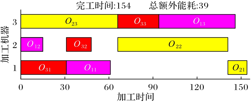
Fig. 2 Gantt chart of individual decoding

Fig. 3 Linear migration model

Fig. 4 Schematic diagram of migration process

Fig. 5 Schematic diagram of processing time resetting operator

Tab. 3 Values of parameters with different levels

参数	第1水平	第2水平	第3水平	第4水平	第5水平
c₁	0.1	0.3	0.5	0.7	0.9
c₂	0.1	0.3	0.5	0.7	0.9
T	0.1	0.2	0.3	0.4	0.5

Tab. 4 Orthogonal experiment table and corresponding average IGD values

实验组	c₁	c₂	T	IGD
1	1	1	1	0.164
2	1	2	2	0.155
3	1	3	3	0.140
4	1	4	4	0.137
5	1	5	5	0.178
6	2	1	2	0.163
7	2	2	3	0.157
8	2	3	4	0.143
9	2	4	5	0.117
10	2	5	1	0.145
11	3	1	3	0.146
12	3	2	4	0.143
13	3	3	5	0.140
14	3	4	1	0.129
15	3	5	2	0.102
16	4	1	4	0.110
17	4	2	5	0.115
18	4	3	1	0.100
19	4	4	2	0.116
20	4	5	3	0.092
21	5	1	5	0.172
22	5	2	1	0.166
23	5	3	2	0.152
24	5	4	3	0.137
25	5	5	4	0.148

Tab. 5 Average IGD values corresponding to parameter levels

参数	第1水平	第2水平	第3水平	第4水平	第5水平
c₁	0.775	0.725	0.660	0.533	0.774
c₂	0.755	0.736	0.675	0.635	0.664
T	0.689	0.687	0.672	0.681	0.722

Tab. 6 Convergence times of other examples

规模	收敛时间/s	规模	收敛时间/s
4×4	30/40/60/80	10×10	400/380/300/320
5×5	80/90/90/90	15×15	380/380/400/450
7×7	120/160/100/200	20×20	400/500/400/450

Fig. 6 Convergence of example 5×5_2

Fig. 7 Boxplots of GD results

Fig. 8 Boxplots of IGD results

Fig. 9 Boxplots of Δ results

Tab. 7 Parameter setting of different algorithms

算法	种群数	交叉概率	变异概率	分区数	外部档案库大小
NSGA-Ⅱ	100	0.7	0.1	—	—
NSGA-Ⅲ	100	0.7	0.1	5	—
SPEA2	100	0.7	0.1	—	100

Tab. 8 Computational results of different algorithms

算例	GD
	Mean				Std
	MOHEA	NSGA-Ⅱ	NSGA-Ⅲ	SPEA2	MOHEA	NSGA-Ⅱ	NSGA-Ⅲ	SPEA2
4×4_1	0.021	0.038	0.040	0.051	0.008	0.013	0.016	0.019
4×4_2	0.039	0.056	0.066	0.070	0.016	0.034	0.024	0.030
4×4_3	0.010	0.024	0.027	0.028	0.010	0.030	0.021	0.021
4×4_4	0.034	0.041	0.051	0.039	0.022	0.024	0.027	0.026
5×5_1	0.040	0.092	0.089	0.081	0.025	0.035	0.050	0.037
5×5_2	0.039	0.045	0.093	0.070	0.020	0.026	0.026	0.020
5×5_3	0.064	0.091	0.081	0.110	0.030	0.028	0.023	0.040
5×5_4	0.059	0.083	0.117	0.094	0.033	0.041	0.043	0.037
7×7_1	0.061	0.114	0.107	0.108	0.028	0.037	0.039	0.033
7×7_2	0.075	0.141	0.117	0.112	0.024	0.043	0.042	0.043
7×7_3	0.056	0.127	0.105	0.156	0.024	0.031	0.026	0.042
7×7_4	0.072	0.137	0.149	0.146	0.034	0.046	0.048	0.033
10×10_1	0.072	0.137	0.169	0.186	0.028	0.040	0.043	0.025
10×10_2	0.076	0.168	0.173	0.176	0.028	0.044	0.039	0.032
10×10_3	0.096	0.160	0.223	0.182	0.030	0.047	0.046	0.038
10×10_4	0.085	0.164	0.181	0.180	0.020	0.027	0.026	0.028
15×15_1	0.076	0.207	0.207	0.187	0.032	0.035	0.028	0.038
15×15_2	0.074	0.202	0.216	0.229	0.035	0.035	0.040	0.034
15×15_3	0.088	0.228	0.206	0.207	0.029	0.043	0.045	0.030
15×15_4	0.061	0.190	0.203	0.166	0.030	0.035	0.049	0.033
20×20_1	0.054	0.196	0.227	0.209	0.018	0.042	0.043	0.036
20×20_2	0.078	0.233	0.226	0.224	0.022	0.053	0.042	0.041
20×20_3	0.054	0.203	0.212	0.233	0.017	0.032	0.030	0.035
20×20_4	0.067	0.215	0.194	0.224	0.018	0.044	0.033	0.036
算例	IGD
	Mean				Std
	MOHEA	NSGA-Ⅱ	NSGA-Ⅲ	SPEA2	MOHEA	NSGA-Ⅱ	NSGA-Ⅲ	SPEA2
4×4_1	0.039	0.089	0.097	0.122	0.016	0.029	0.042	0.051
4×4_2	0.045	0.092	0.103	0.105	0.018	0.026	0.028	0.035
4×4_3	0.033	0.136	0.145	0.137	0.018	0.036	0.041	0.040
4×4_4	0.056	0.112	0.119	0.109	0.031	0.033	0.033	0.024
5×5_1	0.075	0.164	0.153	0.151	0.023	0.041	0.041	0.050
5×5_2	0.066	0.082	0.127	0.099	0.019	0.028	0.023	0.030
5×5_3	0.088	0.153	0.169	0.187	0.041	0.039	0.058	0.052
5×5_4	0.068	0.160	0.156	0.130	0.031	0.032	0.047	0.038
7×7_1	0.110	0.158	0.145	0.136	0.029	0.029	0.037	0.028
7×7_2	0.083	0.159	0.132	0.152	0.016	0.033	0.028	0.043
7×7_3	0.106	0.159	0.150	0.184	0.040	0.022	0.032	0.035
7×7_4	0.097	0.141	0.175	0.162	0.032	0.034	0.032	0.028
10×10_1	0.086	0.141	0.174	0.179	0.018	0.025	0.031	0.022
10×10_2	0.114	0.211	0.216	0.203	0.019	0.038	0.027	0.029
10×10_3	0.111	0.166	0.217	0.166	0.028	0.031	0.031	0.026
10×10_4	0.133	0.184	0.196	0.204	0.034	0.024	0.024	0.024
15×15_1	0.123	0.237	0.238	0.217	0.031	0.029	0.021	0.024
15×15_2	0.138	0.228	0.233	0.252	0.045	0.027	0.032	0.027
15×15_3	0.142	0.250	0.238	0.230	0.025	0.027	0.027	0.019
15×15_4	0.126	0.222	0.238	0.219	0.026	0.022	0.026	0.018
20×20_1	0.104	0.312	0.317	0.311	0.016	0.021	0.020	0.024
20×20_2	0.139	0.301	0.281	0.289	0.022	0.024	0.023	0.025
20×20_3	0.073	0.318	0.308	0.341	0.013	0.018	0.021	0.020
20×20_4	0.128	0.354	0.337	0.355	0.021	0.018	0.021	0.018

Tab. 8 Computational results of different algorithms

算例	GD
	Mean				Std
	MOHEA	NSGA-Ⅱ	NSGA-Ⅲ	SPEA2	MOHEA	NSGA-Ⅱ	NSGA-Ⅲ	SPEA2
4×4_1	0.021	0.038	0.040	0.051	0.008	0.013	0.016	0.019
4×4_2	0.039	0.056	0.066	0.070	0.016	0.034	0.024	0.030
4×4_3	0.010	0.024	0.027	0.028	0.010	0.030	0.021	0.021
4×4_4	0.034	0.041	0.051	0.039	0.022	0.024	0.027	0.026
5×5_1	0.040	0.092	0.089	0.081	0.025	0.035	0.050	0.037
5×5_2	0.039	0.045	0.093	0.070	0.020	0.026	0.026	0.020
5×5_3	0.064	0.091	0.081	0.110	0.030	0.028	0.023	0.040
5×5_4	0.059	0.083	0.117	0.094	0.033	0.041	0.043	0.037
7×7_1	0.061	0.114	0.107	0.108	0.028	0.037	0.039	0.033
7×7_2	0.075	0.141	0.117	0.112	0.024	0.043	0.042	0.043
7×7_3	0.056	0.127	0.105	0.156	0.024	0.031	0.026	0.042
7×7_4	0.072	0.137	0.149	0.146	0.034	0.046	0.048	0.033
10×10_1	0.072	0.137	0.169	0.186	0.028	0.040	0.043	0.025
10×10_2	0.076	0.168	0.173	0.176	0.028	0.044	0.039	0.032
10×10_3	0.096	0.160	0.223	0.182	0.030	0.047	0.046	0.038
10×10_4	0.085	0.164	0.181	0.180	0.020	0.027	0.026	0.028
15×15_1	0.076	0.207	0.207	0.187	0.032	0.035	0.028	0.038
15×15_2	0.074	0.202	0.216	0.229	0.035	0.035	0.040	0.034
15×15_3	0.088	0.228	0.206	0.207	0.029	0.043	0.045	0.030
15×15_4	0.061	0.190	0.203	0.166	0.030	0.035	0.049	0.033
20×20_1	0.054	0.196	0.227	0.209	0.018	0.042	0.043	0.036
20×20_2	0.078	0.233	0.226	0.224	0.022	0.053	0.042	0.041
20×20_3	0.054	0.203	0.212	0.233	0.017	0.032	0.030	0.035
20×20_4	0.067	0.215	0.194	0.224	0.018	0.044	0.033	0.036
算例	IGD
	Mean				Std
	MOHEA	NSGA-Ⅱ	NSGA-Ⅲ	SPEA2	MOHEA	NSGA-Ⅱ	NSGA-Ⅲ	SPEA2
4×4_1	0.039	0.089	0.097	0.122	0.016	0.029	0.042	0.051
4×4_2	0.045	0.092	0.103	0.105	0.018	0.026	0.028	0.035
4×4_3	0.033	0.136	0.145	0.137	0.018	0.036	0.041	0.040
4×4_4	0.056	0.112	0.119	0.109	0.031	0.033	0.033	0.024
5×5_1	0.075	0.164	0.153	0.151	0.023	0.041	0.041	0.050
5×5_2	0.066	0.082	0.127	0.099	0.019	0.028	0.023	0.030
5×5_3	0.088	0.153	0.169	0.187	0.041	0.039	0.058	0.052
5×5_4	0.068	0.160	0.156	0.130	0.031	0.032	0.047	0.038
7×7_1	0.110	0.158	0.145	0.136	0.029	0.029	0.037	0.028
7×7_2	0.083	0.159	0.132	0.152	0.016	0.033	0.028	0.043
7×7_3	0.106	0.159	0.150	0.184	0.040	0.022	0.032	0.035
7×7_4	0.097	0.141	0.175	0.162	0.032	0.034	0.032	0.028
10×10_1	0.086	0.141	0.174	0.179	0.018	0.025	0.031	0.022
10×10_2	0.114	0.211	0.216	0.203	0.019	0.038	0.027	0.029
10×10_3	0.111	0.166	0.217	0.166	0.028	0.031	0.031	0.026
10×10_4	0.133	0.184	0.196	0.204	0.034	0.024	0.024	0.024
15×15_1	0.123	0.237	0.238	0.217	0.031	0.029	0.021	0.024
15×15_2	0.138	0.228	0.233	0.252	0.045	0.027	0.032	0.027
15×15_3	0.142	0.250	0.238	0.230	0.025	0.027	0.027	0.019
15×15_4	0.126	0.222	0.238	0.219	0.026	0.022	0.026	0.018
20×20_1	0.104	0.312	0.317	0.311	0.016	0.021	0.020	0.024
20×20_2	0.139	0.301	0.281	0.289	0.022	0.024	0.023	0.025
20×20_3	0.073	0.318	0.308	0.341	0.013	0.018	0.021	0.020
20×20_4	0.128	0.354	0.337	0.355	0.021	0.018	0.021	0.018

Fig. 10 Pareto frontiers obtained by different algorithms

References 29

1	李振国.基于布谷鸟算法的柔性开放车间调度与方法研究［D］.武汉：华中科技大学， 2019： 1-3.
	LI Z G. Research on flexible open shop scheduling and method based on cuckoo search algorithm［D］. Wuhan： Huazhong University of Science and Technology， 2019： 1-3.
2	ATAN M O， AKTURK M S. Single CNC machine scheduling with controllable processing times and multiple due dates［J］. International Journal of Production Research， 2008， 46（21）： 6087-6111. 10.1080/00207540701262913
3	KAYVANFAR V， KOMAKI G M， AALAEI A， et al. Minimizing total tardiness and earliness on unrelated parallel machines with controllable processing times［J］. Computers and Operations Research， 2014， 41： 31-43. 10.1016/j.cor.2013.08.003
4	王军强，郭银洲，崔福东，等.基于多样性增强的自适应遗传算法的开放式车间调度优化［J］.计算机集成制造系统， 2014， 20（10）： 2479-2493.
	WANG J Q， GUO Y Z， CUI F D， et al. Diversity enhancement-based adaptive genetic algorithm for open-shop scheduling problem［J］. Computer Integrated Manufacturing Systems， 2014， 20（10）： 2479-2493.
5	RAHMANI HOSSEINABADI A A， VAHIDI J， SAEMI B， et al. Extended genetic algorithm for solving open-shop scheduling problem［J］. Soft Computing， 2019， 23（13）： 5099-5116. 10.1007/s00500-018-3177-y
6	SHAREH M B， BARGH S H， RAHMANI HOSSEINABADI A A， et al. An improved bat optimization algorithm to solve the tasks scheduling problem in open shop［J］. Neural Computing and Applications， 2021， 33（5）： 1559-1573. 10.1007/s00521-020-05055-7
7	ABREU L V， CUNHA J O， PRATA B A， et al. A genetic algorithm for scheduling open shops with sequence-dependent setup times［J］. Computers and Operations Research， 2020， 113： No.104793. 10.1016/j.cor.2019.104793
8	MEJÍA G， YURASZECK F. A self-tuning variable neighborhood search algorithm and an effective decoding scheme for open shop scheduling problems with travel/setup times［J］. European Journal of Operational Research， 2020， 285（2）： 484-496. 10.1016/j.ejor.2020.02.010
9	ZHUANG Z L， HUANG Z Z， LU Z Y， et al. An improved artificial bee colony algorithm for solving open shop scheduling problem with two sequence-dependent setup times［J］. Procedia CIRP， 2019， 83： 563-568. 10.1016/j.procir.2019.04.119
10	SHEIKHALISHAHI M， ESKANDARI N， MASHAYEKHI A， et al. Multi-objective open shop scheduling by considering human error and preventive maintenance［J］. Applied Mathematical Modelling， 2019， 67： 573-587. 10.1016/j.apm.2018.11.015
11	SIMON D. Biogeography-based optimization［J］. IEEE Transactions on Evolutionary Computation， 2008， 12（6）： 702-713. 10.1109/tevc.2008.919004
12	黄佳琳，张丫丫，顾幸生.基于改进生物地理学优化算法的分布式装配置换流水车间调度问题［J］.华东理工大学学报（自然科学版）， 2020， 46（6）： 758-769.
	HUANG J L， ZHANG Y Y， GU X S. Distributed assembly permutation flow shop scheduling problem based on modified biogeography-based optimization algorithm［J］. Journal of East China University of Science and Technology， 2020， 46（6）： 758-769.
13	张国辉，聂黎，毛学港.生物地理学算法求解柔性作业车间调度问题［J］.计算机应用研究， 2014， 31（4）： 1005-1008.
	ZHANG G H， NIE L， MAO X G. Solving flexible job-shop scheduling problem based on biogeography-based optimization algorithm［J］. Application Research of Computers， 2014， 31（4）： 1005-1008.
14	WANG Y N， LI X T. A hybrid chaotic biogeography based optimization for the sequence dependent setup times flow-shop scheduling problem with weighted tardiness objective［J］. IEEE Access， 2017， 5： 26046-26062. 10.1109/access.2017.2769100
15	吴定会，孔飞，朱绍文，等.生物地理学算法求解柔性车间作业调度问题［J］.计算机工程与应用， 2015， 51（22）： 206-213， 242. 10.3778/j.issn.1002-8331.1408-0178
	WU D H， KONG F， ZHU S W， et al. Biogeography-based optimization algorithm for flexible job-shop scheduling problems. Computer Engineering and Applications， 2015， 51（22）： 206-213， 242. 10.3778/j.issn.1002-8331.1408-0178
16	XIA H， LI X Y， GAO L. A hybrid genetic algorithm with variable neighborhood search for dynamic integrated process planning and scheduling［J］. Computers and Industrial Engineering， 2016， 102： 99-112. 10.1016/j.cie.2016.10.015
17	YUAN Y， XU H. Flexible job shop scheduling using hybrid differential evolution algorithms［J］. Computers and Industrial Engineering， 2013， 65（2）： 246-260. 10.1016/j.cie.2013.02.022
18	赵诗奎.求解柔性作业车间调度问题的两级邻域搜索混合算法［J］.机械工程学报， 2015， 51（14）： 175-184. 10.3901/jme.2015.14.175
	ZHAO S K. Bilevel neighborhood search hybrid algorithm for the flexible job shop scheduling problem［J］. Journal of Mechanical Engineering， 2015， 51（14）： 175-184. 10.3901/jme.2015.14.175
19	ZHANG G H， GAO L， SHI Y. An effective genetic algorithm for the flexible job-shop scheduling problem［J］. Expert Systems with Applications， 2011， 38（4）： 3563-3573. 10.1016/j.eswa.2010.08.145
20	刘晋伟.并行混沌优化算法及其应用［D］.长沙：湖南大学， 2019： 27-30.
	LIU J W. Improved parallel iterative chaotic optimization algorithm and its application［D］. Changsha： Hunan University， 2019： 27-30.
21	杨德博.基于候鸟优化算法的开放车间调度研究［D］.武汉：华中科技大学， 2017： 15-16， 23-24.
	YANG D B. Research on open shop scheduling based on migrating birds optimization algorithm［D］. Wuhan： Huazhong University of Science and Technology， 2017： 15-16， 23-24.
22	NOWICKI E， SMUTNICKI C. A fast taboo search algorithm for the job shop problem［J］. Management Science， 1996， 42（6）： 797-813. 10.1287/mnsc.42.6.797
23	QIN H B， FAN P F， TANG H T， et al. An effective hybrid discrete grey wolf optimizer for the casting production scheduling problem with multi-objective and multi-constraint［J］. Computers and Industrial Engineering， 2019， 128： 458-476. 10.1016/j.cie.2018.12.061
24	TAILLARD E. Benchmarks for basic scheduling problems［J］. European Journal of Operational Research， 1993， 64（2）： 278-285. 10.1016/0377-2217(93)90182-m
25	DEB K， PRATAP A， AGARWAL S， et al. A fast and elitist multiobjective genetic algorithm： NSGA-II［J］. IEEE Transactions on Evolutionary Computation， 2002， 6（2）： 182-197. 10.1109/4235.996017
26	DEB K， JAIN H. An evolutionary many-objective optimization algorithm using reference-point-based nondominated sorting approach， part I： solving problems with box constraints［J］. IEEE Transactions on Evolutionary Computation， 2014， 18（4）： 577-601. 10.1109/tevc.2013.2281535
27	ZITZLER E， LAUMANNS M， THIELE L. SPEA2： improving the strength pareto evolutionary algorithm ［C］// Proceedings of the EUROGEN 2001 Conference in Athens. Athens， Greece：National Technical University of Athens， 2001： 95-100..
28	张新明，康强，王霞，等.差分迁移和趋优变异的生物地理学优化算法［J］.小型微型计算机系统， 2018， 39（6）： 1168-1177. 10.3969/j.issn.1000-1220.2018.06.010
	ZHANG X M， KANG Q， WANG X， et al. Biogeography-based optimization with differential migration and global-best mutation［J］. Journal of Chinese Computer Systems， 2018， 39（6）： 1168-1177. 10.3969/j.issn.1000-1220.2018.06.010
29	PALUBECKIS G， TOMKEVIČIUS A， OSTREIKA A. Hybridizing simulated annealing with variable neighborhood search for bipartite graph crossing minimization［J］. Applied Mathematics and Computation， 2019， 348： 84-101. 10.1016/j.amc.2018.11.051

[1]	CHEN Linfeng, QI Xuemei, CHEN Junwen, HUANG Cheng, CHEN Fulong. Quantum-inspired migrating birds co-optimization algorithm for lot-streaming flow shop scheduling problem [J]. Journal of Computer Applications, 2019, 39(11): 3250-3256.
[2]	QI Xuemei, WANG Hongtao, CHEN Fulong, TANG Qimei, SUN Yunxiang. Novel quantum differential evolutionary algorithm for blocking flowshop scheduling [J]. Journal of Computer Applications, 2015, 35(3): 663-667.
[3]	PAN Yuxia XIE Guang XIAO Heng. Discrete harmony search algorithm for lot-streaming flow shop scheduling problem with setup time [J]. Journal of Computer Applications, 2014, 34(2): 528-532.
[4]	LI Xiaobin BAI Yan GENG Linxiao. Improved genetic algorithm for solving permutation flow shop scheduling problem [J]. Journal of Computer Applications, 2013, 33(12): 3576-3579.
[5]	. Relationship between makespan of grid job and granularity of job partitioning [J]. Journal of Computer Applications, 2011, 31(02): 530-532.
[6]	. Workflow scheduling algorithm based on load balance in grid [J]. Journal of Computer Applications, 2010, 30(12): 3184-3186.
[7]	. Scheduling algorithm on grid resources in consideration of local workloads [J]. Journal of Computer Applications, 2010, 30(11): 2861-2863.

Multi-objective hybrid evolutionary algorithm for solving open-shop scheduling problem with controllable processing time

多目标混合进化算法求解加工时间可控的开放车间调度问题

RichHTML

PDF

Knowledge

Abstract

Cite this article

share this article

Figures/Tables 18

References 29

Related Articles 7

Recommended Articles

Metrics