


《计算机应用》唯一官方网站 ›› 2024, Vol. 44 ›› Issue (8): 2643-2650.DOI: 10.11772/j.issn.1001-9081.2023081169
• 前沿与综合应用 • 上一篇
石乾宏1, 杨燕1( ), 江永全1, 欧阳小草1, 范武波2, 陈强2, 姜涛2, 李媛2
收稿日期:2023-08-31
修回日期:2023-09-11
接受日期:2023-10-09
发布日期:2024-08-22
出版日期:2024-08-10
通讯作者:
杨燕
作者简介:石乾宏(1999—),男,河南荥阳人,硕士研究生,主要研究方向:数据挖掘、序列数据分析基金资助:
Qianhong SHI1, Yan YANG1(), Yongquan JIANG1, Xiaocao OUYANG1, Wubo FAN2, Qiang CHEN2, Tao JIANG2, Yuan LI2
Received:2023-08-31
Revised:2023-09-11
Accepted:2023-10-09
Online:2024-08-22
Published:2024-08-10
Contact:
Yan YANG
About author:SHI Qianhong, born in 1999, M. S. candidate. His research interests include data mining, sequential data analysis.Supported by:摘要:
空气质量数据作为一种典型的时空数据,具有复杂的多尺度内在特性并存在突变的问题。针对现有空气质量预测方法在处理包含大量突变数据的空气质量预测任务时表现不佳的问题,提出一种面向空气质量预测的多粒度突变拟合网络(MACFN)。首先,针对空气质量数据在时间上的周期性,对输入数据进行了多粒度的特征提取。然后,采用图卷积网络与时间卷积网络分别提取空气质量数据的空间关联性与时间依赖性。最后,设计一个突变拟合网络自适应地学习数据中的突变部分,从而减小预测误差。所提网络在3个真实的空气质量数据集上进行了实验评估,与多尺度时空网络(MSSTN)相比,均方根误差(RMSE)分别下降约11.6%、6.3%和2.2%。实验结果表明,MACFN能有效捕捉复杂的时空关系,并在变化幅度较大、易发生突变的空气质量预测任务中有更好表现。
中图分类号:
石乾宏, 杨燕, 江永全, 欧阳小草, 范武波, 陈强, 姜涛, 李媛. 面向空气质量预测的多粒度突变拟合网络[J]. 计算机应用, 2024, 44(8): 2643-2650.
Qianhong SHI, Yan YANG, Yongquan JIANG, Xiaocao OUYANG, Wubo FAN, Qiang CHEN, Tao JIANG, Yuan LI. Multi-granularity abrupt change fitting network for air quality prediction[J]. Journal of Computer Applications, 2024, 44(8): 2643-2650.
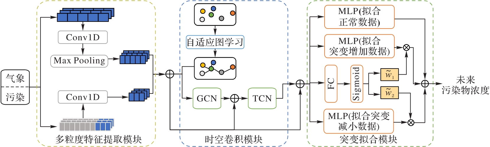
图1 MACFN的整体框架
Fig. 1 Overall framework of MACFN
| 数据集 | 监测站点数 | PM2.5浓度平均值 | PM2.5浓度标准差 |
|---|---|---|---|
| 北京 | 35 | 84.20 | 82.53 |
| 天津 | 24 | 80.21 | 66.32 |
| 深圳 | 11 | 33.02 | 22.18 |
表1 实验数据集详情
Tab. 1 Details of experiment datasets
| 数据集 | 监测站点数 | PM2.5浓度平均值 | PM2.5浓度标准差 |
|---|---|---|---|
| 北京 | 35 | 84.20 | 82.53 |
| 天津 | 24 | 80.21 | 66.32 |
| 深圳 | 11 | 33.02 | 22.18 |
| 模型 | 网络平均 训练时间 | 模型 | 网络平均 训练时间 |
|---|---|---|---|
| LSTM | 6 | PM2.5-GNN | 76 |
| NSTransformers | 43 | Deep-AIR | 61 |
| DCRNN | 63 | MACFN | 92 |
| MSSTN | 87 |
表2 各相关模型单轮训练时间比较 (s)
Tab. 2 Comparison of single round training time among related models
| 模型 | 网络平均 训练时间 | 模型 | 网络平均 训练时间 |
|---|---|---|---|
| LSTM | 6 | PM2.5-GNN | 76 |
| NSTransformers | 43 | Deep-AIR | 61 |
| DCRNN | 63 | MACFN | 92 |
| MSSTN | 87 |
| 模型 | 3 h | 6 h | 12 h | 24 h | ||||||||
|---|---|---|---|---|---|---|---|---|---|---|---|---|
| MAE | RMSE | R² | MAE | RMSE | R² | MAE | RMSE | R² | MAE | RMSE | R² | |
| LSTM | 35.21 | 57.39 | 0.39 | 39.12 | 61.71 | 0.31 | 45.16 | 67.68 | 0.17 | 52.19 | 75.69 | 0.01 |
| NSTransformers | 23.58 | 41.53 | 0.69 | 32.80 | 54.36 | 0.47 | 44.87 | 65.90 | 0.23 | 50.46 | 71.96 | 0.09 |
| DCRNN | 26.67 | 47.92 | 0.57 | 34.88 | 56.74 | 0.42 | 44.76 | 66.37 | 0.21 | 52.02 | 75.35 | 0.01 |
| MSSTN | 23.01 | 41.33 | 0.69 | 33.80 | 53.83 | 0.47 | 43.66 | 64.93 | 0.25 | 50.40 | 72.78 | 0.05 |
| PM2.5-GNN | 24.73 | 43.26 | 0.67 | 34.39 | 55.09 | 0.44 | 43.44 | 65.73 | 0.23 | 51.78 | 74.92 | 0.02 |
| Deep-AIR | 22.52 | 40.80 | 0.71 | 32.89 | 53.61 | 0.47 | 43.83 | 65.42 | 0.25 | 50.30 | 72.52 | 0.06 |
| MACFN | 21.01 | 35.81 | 0.78 | 30.38 | 46.44 | 0.58 | 39.91 | 57.35 | 0.39 | 46.86 | 67.44 | 0.13 |
表3 在北京数据集上MACFN和基线模型的性能比较
Tab. 3 Performance comparison of MACFN and baseline models on Beijing dataset
| 模型 | 3 h | 6 h | 12 h | 24 h | ||||||||
|---|---|---|---|---|---|---|---|---|---|---|---|---|
| MAE | RMSE | R² | MAE | RMSE | R² | MAE | RMSE | R² | MAE | RMSE | R² | |
| LSTM | 35.21 | 57.39 | 0.39 | 39.12 | 61.71 | 0.31 | 45.16 | 67.68 | 0.17 | 52.19 | 75.69 | 0.01 |
| NSTransformers | 23.58 | 41.53 | 0.69 | 32.80 | 54.36 | 0.47 | 44.87 | 65.90 | 0.23 | 50.46 | 71.96 | 0.09 |
| DCRNN | 26.67 | 47.92 | 0.57 | 34.88 | 56.74 | 0.42 | 44.76 | 66.37 | 0.21 | 52.02 | 75.35 | 0.01 |
| MSSTN | 23.01 | 41.33 | 0.69 | 33.80 | 53.83 | 0.47 | 43.66 | 64.93 | 0.25 | 50.40 | 72.78 | 0.05 |
| PM2.5-GNN | 24.73 | 43.26 | 0.67 | 34.39 | 55.09 | 0.44 | 43.44 | 65.73 | 0.23 | 51.78 | 74.92 | 0.02 |
| Deep-AIR | 22.52 | 40.80 | 0.71 | 32.89 | 53.61 | 0.47 | 43.83 | 65.42 | 0.25 | 50.30 | 72.52 | 0.06 |
| MACFN | 21.01 | 35.81 | 0.78 | 30.38 | 46.44 | 0.58 | 39.91 | 57.35 | 0.39 | 46.86 | 67.44 | 0.13 |
| 模型 | 3 h | 6 h | 12 h | 24 h | ||||||||
|---|---|---|---|---|---|---|---|---|---|---|---|---|
| MAE | RMSE | R² | MAE | RMSE | R² | MAE | RMSE | R² | MAE | RMSE | R² | |
| LSTM | 27.56 | 38.89 | 0.19 | 29.93 | 41.50 | 0.14 | 33.77 | 43.72 | 0.06 | 34.86 | 44.72 | 0.01 |
| NSTransformers | 17.39 | 27.03 | 0.62 | 23.30 | 34.15 | 0.40 | 29.55 | 40.88 | 0.15 | 33.51 | 44.85 | 0.01 |
| DCRNN | 17.96 | 27.51 | 0.60 | 24.01 | 35.23 | 0.34 | 31.02 | 42.80 | 0.08 | 34.55 | 44.75 | 0.01 |
| MSSTN | 16.76 | 26.28 | 0.63 | 23.07 | 33.90 | 0.41 | 30.15 | 40.57 | 0.16 | 33.97 | 43.96 | 0.01 |
| PM2.5-GNN | 17.63 | 27.39 | 0.61 | 23.45 | 34.36 | 0.39 | 30.37 | 41.38 | 0.12 | 34.25 | 45.83 | 0.01 |
| Deep-AIR | 17.39 | 26.94 | 0.61 | 23.54 | 34.85 | 0.38 | 29.72 | 41.19 | 0.13 | 33.96 | 44.29 | 0.01 |
| MACFN | 16.63 | 24.32 | 0.68 | 22.31 | 30.56 | 0.47 | 28.17 | 37.94 | 0.29 | 33.49 | 43.41 | 0.03 |
表4 在天津数据集上MACFN和基线模型的性能比较
Tab. 4 Performance comparison of MACFN and baseline models on Tianjin dataset
| 模型 | 3 h | 6 h | 12 h | 24 h | ||||||||
|---|---|---|---|---|---|---|---|---|---|---|---|---|
| MAE | RMSE | R² | MAE | RMSE | R² | MAE | RMSE | R² | MAE | RMSE | R² | |
| LSTM | 27.56 | 38.89 | 0.19 | 29.93 | 41.50 | 0.14 | 33.77 | 43.72 | 0.06 | 34.86 | 44.72 | 0.01 |
| NSTransformers | 17.39 | 27.03 | 0.62 | 23.30 | 34.15 | 0.40 | 29.55 | 40.88 | 0.15 | 33.51 | 44.85 | 0.01 |
| DCRNN | 17.96 | 27.51 | 0.60 | 24.01 | 35.23 | 0.34 | 31.02 | 42.80 | 0.08 | 34.55 | 44.75 | 0.01 |
| MSSTN | 16.76 | 26.28 | 0.63 | 23.07 | 33.90 | 0.41 | 30.15 | 40.57 | 0.16 | 33.97 | 43.96 | 0.01 |
| PM2.5-GNN | 17.63 | 27.39 | 0.61 | 23.45 | 34.36 | 0.39 | 30.37 | 41.38 | 0.12 | 34.25 | 45.83 | 0.01 |
| Deep-AIR | 17.39 | 26.94 | 0.61 | 23.54 | 34.85 | 0.38 | 29.72 | 41.19 | 0.13 | 33.96 | 44.29 | 0.01 |
| MACFN | 16.63 | 24.32 | 0.68 | 22.31 | 30.56 | 0.47 | 28.17 | 37.94 | 0.29 | 33.49 | 43.41 | 0.03 |
| 模型 | 3 h | 6 h | 12 h | 24 h | ||||||||
|---|---|---|---|---|---|---|---|---|---|---|---|---|
| MAE | RMSE | R² | MAE | RMSE | R² | MAE | RMSE | R² | MAE | RMSE | R² | |
| LSTM | 8.98 | 12.35 | 0.21 | 9.89 | 13.40 | 0.11 | 10.72 | 14.26 | 0.02 | 12.29 | 15.82 | 0.02 |
| NSTransformers | 5.72 | 8.74 | 0.64 | 7.84 | 11.23 | 0.38 | 9.59 | 13.25 | 0.14 | 10.24 | 13.74 | 0.06 |
| DCRNN | 6.01 | 9.16 | 0.59 | 8.48 | 12.14 | 0.28 | 10.22 | 14.01 | 0.05 | 11.29 | 14.90 | 0.01 |
| MSSTN | 5.90 | 8.75 | 0.64 | 8.13 | 11.45 | 0.35 | 9.88 | 13.54 | 0.10 | 10.71 | 14.15 | 0.01 |
| PM2.5-GNN | 5.89 | 8.96 | 0.61 | 8.28 | 11.94 | 0.30 | 9.85 | 13.53 | 0.11 | 11.00 | 14.65 | 0.01 |
| Deep-AIR | 5.85 | 8.77 | 0.63 | 8.23 | 11.67 | 0.33 | 9.98 | 13.59 | 0.10 | 10.90 | 14.50 | 0.01 |
| MACFN | 5.83 | 8.73 | 0.63 | 7.94 | 11.19 | 0.39 | 9.42 | 13.13 | 0.16 | 10.19 | 13.71 | 0.06 |
表5 在深圳数据集上MACFN和基线模型的性能比较
Tab. 5 Performance comparison of MACFN and baseline models on Shenzhen dataset
| 模型 | 3 h | 6 h | 12 h | 24 h | ||||||||
|---|---|---|---|---|---|---|---|---|---|---|---|---|
| MAE | RMSE | R² | MAE | RMSE | R² | MAE | RMSE | R² | MAE | RMSE | R² | |
| LSTM | 8.98 | 12.35 | 0.21 | 9.89 | 13.40 | 0.11 | 10.72 | 14.26 | 0.02 | 12.29 | 15.82 | 0.02 |
| NSTransformers | 5.72 | 8.74 | 0.64 | 7.84 | 11.23 | 0.38 | 9.59 | 13.25 | 0.14 | 10.24 | 13.74 | 0.06 |
| DCRNN | 6.01 | 9.16 | 0.59 | 8.48 | 12.14 | 0.28 | 10.22 | 14.01 | 0.05 | 11.29 | 14.90 | 0.01 |
| MSSTN | 5.90 | 8.75 | 0.64 | 8.13 | 11.45 | 0.35 | 9.88 | 13.54 | 0.10 | 10.71 | 14.15 | 0.01 |
| PM2.5-GNN | 5.89 | 8.96 | 0.61 | 8.28 | 11.94 | 0.30 | 9.85 | 13.53 | 0.11 | 11.00 | 14.65 | 0.01 |
| Deep-AIR | 5.85 | 8.77 | 0.63 | 8.23 | 11.67 | 0.33 | 9.98 | 13.59 | 0.10 | 10.90 | 14.50 | 0.01 |
| MACFN | 5.83 | 8.73 | 0.63 | 7.94 | 11.19 | 0.39 | 9.42 | 13.13 | 0.16 | 10.19 | 13.71 | 0.06 |
| 模型 | 3 h | 6 h | 12 h | 24 h | ||||||||
|---|---|---|---|---|---|---|---|---|---|---|---|---|
| MAE | RMSE | R² | MAE | RMSE | R² | MAE | RMSE | R² | MAE | RMSE | R² | |
| MACFN-ng | 22.66 | 37.04 | 0.72 | 31.60 | 48.06 | 0.53 | 40.72 | 58.69 | 0.31 | 47.74 | 68.07 | 0.08 |
| MACFN-nt | 23.34 | 38.55 | 0.71 | 31.14 | 49.04 | 0.53 | 40.32 | 59.23 | 0.33 | 48.68 | 68.82 | 0.09 |
| MACFN-ns | 22.94 | 40.80 | 0.67 | 33.45 | 53.06 | 0.47 | 43.57 | 64.80 | 0.28 | 49.95 | 73.76 | 0.04 |
| MACFN-no | 21.74 | 36.65 | 0.73 | 30.89 | 47.37 | 0.55 | 40.94 | 59.66 | 0.30 | 50.19 | 70.53 | 0.09 |
| MACFN-nm1 | 21.94 | 36.73 | 0.73 | 31.07 | 46.52 | 0.56 | 40.62 | 58.82 | 0.32 | 48.77 | 67.17 | 0.11 |
| MACFN-nm2 | 21.73 | 36.53 | 0.73 | 31.03 | 46.69 | 0.56 | 40.45 | 58.23 | 0.33 | 49.54 | 68.33 | 0.08 |
| MACFN-nm3 | 21.86 | 36.48 | 0.73 | 31.62 | 46.74 | 0.54 | 40.68 | 57.87 | 0.35 | 48.61 | 68.95 | 0.08 |
| MACFN | 21.01 | 35.81 | 0.78 | 30.38 | 46.44 | 0.58 | 39.91 | 57.35 | 0.39 | 46.86 | 67.44 | 0.13 |
表6 变体模型与MACFN的性能比较
Tab. 6 Performance comparison of variant models with MACFN
| 模型 | 3 h | 6 h | 12 h | 24 h | ||||||||
|---|---|---|---|---|---|---|---|---|---|---|---|---|
| MAE | RMSE | R² | MAE | RMSE | R² | MAE | RMSE | R² | MAE | RMSE | R² | |
| MACFN-ng | 22.66 | 37.04 | 0.72 | 31.60 | 48.06 | 0.53 | 40.72 | 58.69 | 0.31 | 47.74 | 68.07 | 0.08 |
| MACFN-nt | 23.34 | 38.55 | 0.71 | 31.14 | 49.04 | 0.53 | 40.32 | 59.23 | 0.33 | 48.68 | 68.82 | 0.09 |
| MACFN-ns | 22.94 | 40.80 | 0.67 | 33.45 | 53.06 | 0.47 | 43.57 | 64.80 | 0.28 | 49.95 | 73.76 | 0.04 |
| MACFN-no | 21.74 | 36.65 | 0.73 | 30.89 | 47.37 | 0.55 | 40.94 | 59.66 | 0.30 | 50.19 | 70.53 | 0.09 |
| MACFN-nm1 | 21.94 | 36.73 | 0.73 | 31.07 | 46.52 | 0.56 | 40.62 | 58.82 | 0.32 | 48.77 | 67.17 | 0.11 |
| MACFN-nm2 | 21.73 | 36.53 | 0.73 | 31.03 | 46.69 | 0.56 | 40.45 | 58.23 | 0.33 | 49.54 | 68.33 | 0.08 |
| MACFN-nm3 | 21.86 | 36.48 | 0.73 | 31.62 | 46.74 | 0.54 | 40.68 | 57.87 | 0.35 | 48.61 | 68.95 | 0.08 |
| MACFN | 21.01 | 35.81 | 0.78 | 30.38 | 46.44 | 0.58 | 39.91 | 57.35 | 0.39 | 46.86 | 67.44 | 0.13 |
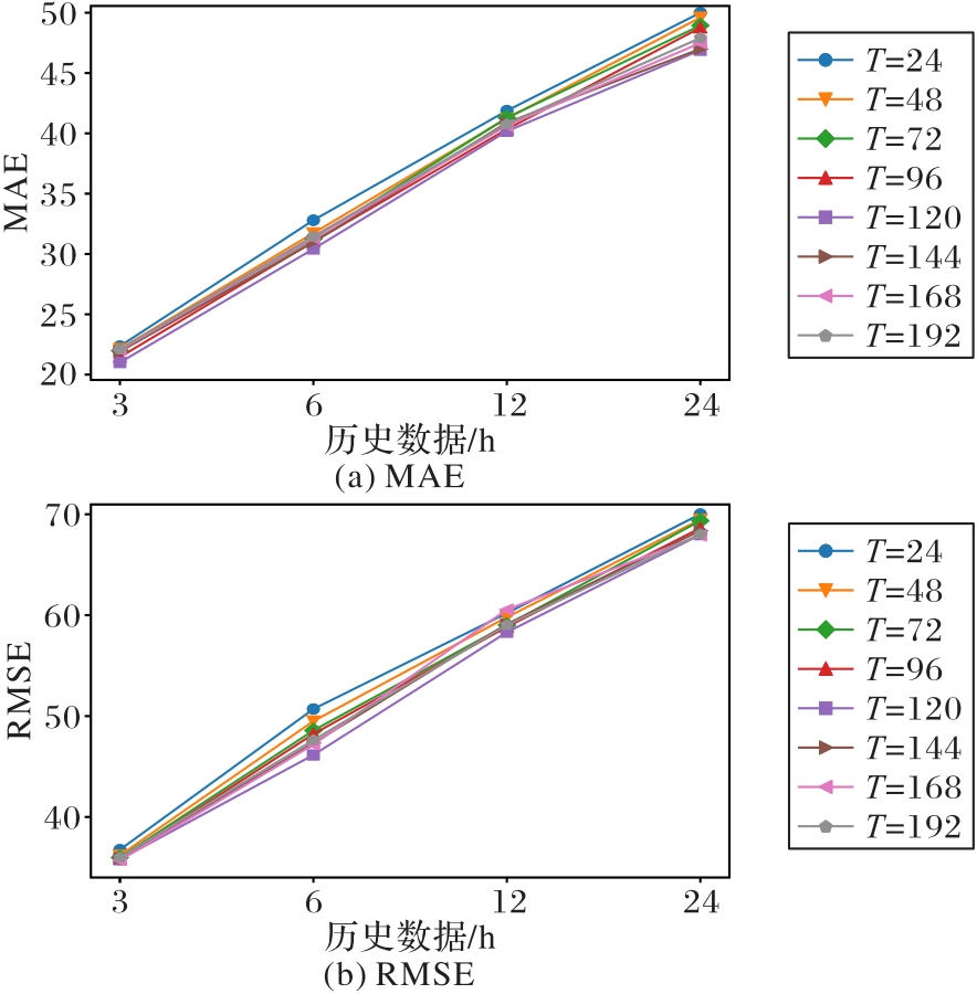
图2 MACFN中不同长度历史数据对北京数据集的影响
Fig. 2 Impact of different lengths of historical data in MACFN on Beijing dataset
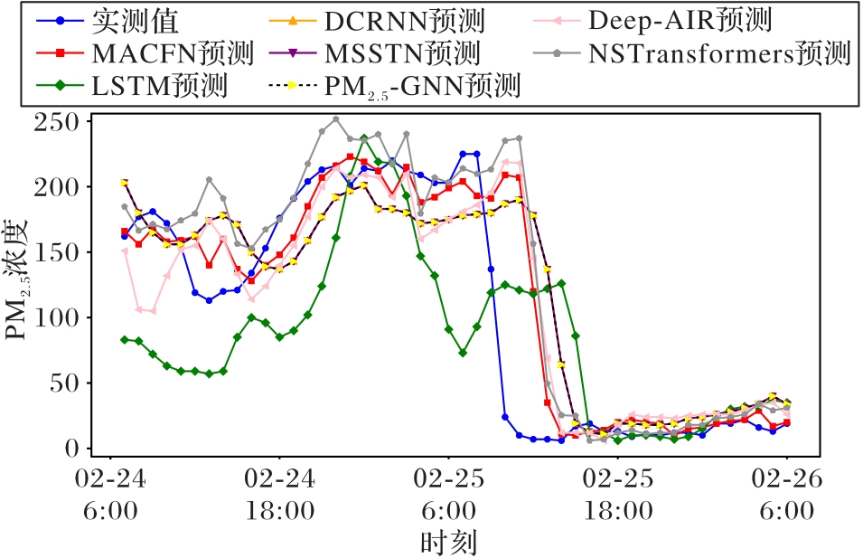
图3 不同模型预测3 h后北京通州站点PM2.5浓度曲线(2015年)
Fig. 3 PM2.5 concentration curves of Tongzhou site in Beijing after three hours predicted by different models (2015)
| 1 | FULLER R, LANDRIGAN P J, BALAKRISHNAN K, et al. Pollution and health: a progress update[J]. The Lancet Planetary Health, 2022, 6(6): e535-e547. |
| 2 | 王志娟,韩力慧,陈旭锋,等.北京典型污染过程PM2.5的特性和来源[J].安全与环境学报, 2012,12(5):122-126. |
| WANG Z J, HAN L H, CHEN X F, et al. Characteristics and sources of PM2.5 in typical atmospheric pollution episodes in Beijing[J]. Journal of Safety and Environment, 2012,12(5): 122-126. | |
| 3 | 陈军,高岩,张烨培,等. PM2.5扩散模型及预测研究[J]. 数学的实践与认识, 2014, 44(15): 16-27. |
| CHEN J, GAO Y, ZHANG Y P, al at. Study on the diffusion model and forecast of PM2.5 pollution[J]. Mathematics in Practice and Theory, 2014, 44(15): 16-27. | |
| 4 | ZHANG L, LIN J, QIU R, et al. Trend analysis and forecast of PM2.5 in Fuzhou, China using the ARIMA model[J]. Ecological Indicators, 2018, 95: 702-710. |
| 5 | LIU T, LAU A K H, SANDBRINK K, et al. Time series forecasting of air quality based on regional numerical modeling in Hong Kong[J]. Journal of Geophysical Research: Atmospheres, 2018, 123(8): 4175-4196. |
| 6 | LIU H, YAN G, DUAN Z, et al. Intelligent modeling strategies for forecasting air quality time series: a review[J]. Applied Soft Computing, 2021, 102: 106957. |
| 7 | YANG L, QIN C, LI K, et al. Quantifying the spatiotemporal heterogeneity of PM2.5 pollution and its determinants in 273 cities in China[J]. International Journal of Environmental Research and Public Health, 2023, 20(2): 1183. |
| 8 | 王振波,方创琳,许光,等. 2014年中国城市PM2.5浓度的时空变化规律[J].地理学报, 2015, 70(11):1720-1734. |
| WANG Z B, FANG C L, XU G, et al. Spatial-temporal characteristics of the PM2.5 in China in 2014[J]. Acta Geographica Sinica, 2015, 70(11): 1720-1734. | |
| 9 | HUANG P, ZHANG J, TANG Y, et al. Spatial and temporal distribution of PM2.5 pollution in Xi’an city, China[J]. International Journal of Environmental Research and Public Health, 2015, 12(6): 6608-6625. |
| 10 | LOGANATHAN N, RAHIM Y I. Forecasting international tourism demand in Malaysia using Box Jenkins SARIMA application[J]. South Asian Journal of Tourism and Heritage, 2010, 3(2): 50-60. |
| 11 | KUMAR A, GOYAL P. Forecasting of daily air quality index in Delhi[J]. Science of the Total Environment, 2011, 409(24): 5517-5523. |
| 12 | MAHALINGAM U, ELANGOVAN K, DOBHAL H, et al. A machine learning model for air quality prediction for smart cities[C]// Proceedings of the 2019 International Conference on Wireless Communications Signal Processing and Networking. Piscataway: IEEE, 2019: 452-457. |
| 13 | LI X, LUO A, LI J, et al. Air pollutant concentration forecast based on support vector regression and quantum-behaved particle swarm optimization[J]. Environmental Modeling & Assessment, 2019, 24(6): 205-222. |
| 14 | KETU S. Spatial air quality index and air pollutant concentration prediction using linear regression based Recursive Feature Elimination with Random Forest Regression (RFERF): a case study in India[J]. Natural Hazards, 2022, 114(4):2109-2138. |
| 15 | ZHAO X, ZHANG R, WU J-L, et al. A deep recurrent neural network for air quality classification[J]. Journal of Information Hiding and Multimedia Signal Processing, 2018, 9(2):346-354. |
| 16 | Y-T TSAI, ZENG Y-R, CHANG Y-S. Air pollution forecasting using RNN with LSTM[C]// Proceedings of the 2018 IEEE 16th International Conference on Dependable, Autonomic and Secure Computing, 16th International Conference on Pervasive Intelligence and Computing, 4th International Conference on Big Data Intelligence and Computer and Cyber Science and Technology Congress. Piscataway: IEEE, 2018: 1074-1079. |
| 17 | LIU Y, WU H, WANG J, et al. Non-stationary transformers: exploring the stationarity in time series forecasting[J]. Advances in Neural Information Processing Systems, 2022, 35: 9881-9893. |
| 18 | KIM T-Y, CHO S-B. Predicting residential energy consumption using CNN-LSTM neural networks[J]. Energy, 2019, 182: 72-81. |
| 19 | CHENG W, SHEN Y, ZHU Y, et al. A neural attention model for urban air quality inference: learning the weights of monitoring stations[J]. Proceedings of the AAAI Conference on Artificial Intelligence, 2018, 32(1): 2151-2158. |
| 20 | DU S, LI T, YANG Y, et al. Deep air quality forecasting using hybrid deep learning framework[J]. IEEE Transactions on Knowledge and Data Engineering, 2019, 33(6): 2412-2424. |
| 21 | GILMER J, SCHOENHOLZ S S, RILEY P F, et al. Neural message passing for Quantum chemistry[C]// Proceedings of the 34th International Conference on Machine Learning. New York: JMLR.org, 2017: 1263-1272. |
| 22 | VELICČKOVIĆ P, CUCURULL G, CASANOVA A, et al. Graph attention networks[EB/OL]. (2017-10-30)[2023-06-29]. . |
| 23 | WU L, LIN H, TAN C, et al. Self-supervised learning on graphs: contrastive, generative, or predictive[J]. IEEE Transactions on Knowledge and Data Engineering, 2023, 35(4): 4216-4235. |
| 24 | LI Y, YU R, SHAHABI C, et al. Diffusion convolutional recurrent neural network: data-driven traffic forecasting[EB/OL]. (2017-07-06) [2023-06-29]. . |
| 25 | WU Z, WANG Y, ZHANG L. MSSTN: multi-scale spatial temporal network for air pollution prediction[C]// Proceedings of the 2019 IEEE International Conference on Big Data. Piscataway: IEEE, 2019: 1547-1556. |
| 26 | WU Z, PAN S, LONG G, et al. Graph WaveNet for deep spatial-temporal graph modeling[C]// Proceedings of the 28th International Joint Conference on Artificial Intelligence. Palo Alto: AAAI Press, 2019: 1907-1913. |
| 27 | WANG S, LI Y, ZHANG J, et al. PM2.5-GNN: a domain knowledge enhanced graph neural network for PM2.5 forecasting[C]// Proceedings of the 28th International Conference on Advances in Geographic Information Systems. New York: ACM, 2020: 163-166. |
| 28 | ZHOU W, WANG H, ZHANG Y, et al. Multi-scale progressive gated Transformer for physiological signal classification[C]// Proceedings of the 14th Asian Conference on Machine Learning. New York: JMLR.org, 2023: 1293-1308. |
| 29 | GAO L, WANG T, REN X, et al. Impact of atmospheric quasi-biweekly oscillation on the persistent heavy PM2.5 pollution over Beijing-Tianjin-Hebei region, China during winter[J]. Atmospheric Research, 2020, 242: 105017. |
| 30 | ZHOU H, ZHANG S, PENG J, et al. Informer:beyond efficient transformer for long sequence time-series forecasting[J]. Proceedings of the AAAI Conference on Artificial Intelligence, 2021, 35(12): 11106-11115. |
| 31 | HE K, ZHANG X, REN S, et al. Identity mappings in deep residual networks[C]// Proceedings of the 2016 European Conference on Computer Vision. Cham: Springer, 2016: 630-645. |
| 32 | GIRSHICK R. Fast R-CNN[C]// Proceedings of the 2015 IEEE International Conference on Computer Vision. Piscataway: IEEE, 2015: 1440-1448. |
| 33 | ZHENG Y, YI X, LI M, et al. Forecasting fine-grained air quality based on big data[C]// Proceedings of the 21th ACM SIGKDD International Conference on Knowledge Discovery and Data Mining. New York: ACM, 2015: 2267-2276. |
| [1] | 李顺勇, 李师毅, 胥瑞, 赵兴旺. 基于自注意力融合的不完整多视图聚类算法[J]. 《计算机应用》唯一官方网站, 2024, 44(9): 2696-2703. |
| [2] | 黄云川, 江永全, 黄骏涛, 杨燕. 基于元图同构网络的分子毒性预测[J]. 《计算机应用》唯一官方网站, 2024, 44(9): 2964-2969. |
| [3] | 杨鑫, 陈雪妮, 吴春江, 周世杰. 结合变种残差模型和Transformer的城市公路短时交通流预测[J]. 《计算机应用》唯一官方网站, 2024, 44(9): 2947-2951. |
| [4] | 秦璟, 秦志光, 李发礼, 彭悦恒. 基于概率稀疏自注意力神经网络的重性抑郁疾患诊断[J]. 《计算机应用》唯一官方网站, 2024, 44(9): 2970-2974. |
| [5] | 王熙源, 张战成, 徐少康, 张宝成, 罗晓清, 胡伏原. 面向手术导航3D/2D配准的无监督跨域迁移网络[J]. 《计算机应用》唯一官方网站, 2024, 44(9): 2911-2918. |
| [6] | 潘烨新, 杨哲. 基于多级特征双向融合的小目标检测优化模型[J]. 《计算机应用》唯一官方网站, 2024, 44(9): 2871-2877. |
| [7] | 刘禹含, 吉根林, 张红苹. 基于骨架图与混合注意力的视频行人异常检测方法[J]. 《计算机应用》唯一官方网站, 2024, 44(8): 2551-2557. |
| [8] | 顾焰杰, 张英俊, 刘晓倩, 周围, 孙威. 基于时空多图融合的交通流量预测[J]. 《计算机应用》唯一官方网站, 2024, 44(8): 2618-2625. |
| [9] | 赵亦群, 张志禹, 董雪. 基于密集残差物理信息神经网络的各向异性旅行时计算方法[J]. 《计算机应用》唯一官方网站, 2024, 44(7): 2310-2318. |
| [10] | 徐松, 张文博, 王一帆. 基于时空信息的轻量视频显著性目标检测网络[J]. 《计算机应用》唯一官方网站, 2024, 44(7): 2192-2199. |
| [11] | 刘瑞华, 郝子赫, 邹洋杨. 基于多层级精细特征融合的步态识别算法[J]. 《计算机应用》唯一官方网站, 2024, 44(7): 2250-2257. |
| [12] | 孙逊, 冯睿锋, 陈彦如. 基于深度与实例分割融合的单目3D目标检测方法[J]. 《计算机应用》唯一官方网站, 2024, 44(7): 2208-2215. |
| [13] | 吴筝, 程志友, 汪真天, 汪传建, 王胜, 许辉. 基于深度学习的患者麻醉复苏过程中的头部运动幅度分类方法[J]. 《计算机应用》唯一官方网站, 2024, 44(7): 2258-2263. |
| [14] | 李欢欢, 黄添强, 丁雪梅, 罗海峰, 黄丽清. 基于多尺度时空图卷积网络的交通出行需求预测[J]. 《计算机应用》唯一官方网站, 2024, 44(7): 2065-2072. |
| [15] | 张郅, 李欣, 叶乃夫, 胡凯茜. 基于暗知识保护的模型窃取防御技术DKP[J]. 《计算机应用》唯一官方网站, 2024, 44(7): 2080-2086. |
| 阅读次数 | ||||||
|
全文 |
|
|||||
|
摘要 |
|
|||||