


《计算机应用》唯一官方网站 ›› 2026, Vol. 46 ›› Issue (10): 3206-3214.DOI: 10.11772/j.issn.1001-9081.2025080971
• 数据科学与技术 • 上一篇
刘晟1, 童英华1,2( )
收稿日期:2025-08-25
修回日期:2025-09-11
接受日期:2025-09-29
发布日期:2025-11-07
出版日期:2026-10-10
通讯作者:
童英华
作者简介:刘晟(1998—),男,江西吉安人,硕士研究生,CCF会员,主要研究方向:物联网系统的可靠性、深度学习
基金资助:
Sheng LIU1, Yinghua TONG1,2()
Received:2025-08-25
Revised:2025-09-11
Accepted:2025-09-29
Online:2025-11-07
Published:2026-10-10
Contact:
Yinghua TONG
About author:LIU Sheng, born in 1998, M. S. candidate. His research interests include IoT system reliability, deep learning.
Supported by:摘要:
针对现有Transformer类模型在趋势性信息提取方面存在的不足,以及传感器异构性导致的变量相关性建模失真等问题,提出一种基于转置自注意力机制(TSA)与卷积自编码器(CAE)的多元时序数据分析方法。该方法通过构建转置一维CAE结构,从时间维度实现时序数据的特征重建,有效捕获多元时序数据中的长期趋势信息;同时,将TSA机制引入多变量相关性分析过程,显著提升变量间关联关系的建模精度。与近年主流方法的预测性能对比实验结果表明,所提方法的平均均方误差(MSE)为0.545,相较于iTransformer和DLinear分别降低了11.4%和7.4%。此外,在5个公共数据集上的异常检测实验结果表明,该方法的平均F1分数为84.92%,优于所有基线方法。在真实水质监测数据集上的预测实验结果表明,所提方法的平均绝对误差(MAE)和MSE相较于Autoformer分别降低了46.2%和42.9%,验证了该方法在实际应用场景中的有效性。
中图分类号:
刘晟, 童英华. 基于转置自注意力机制与卷积自编码器的多元时序数据分析方法[J]. 计算机应用, 2026, 46(10): 3206-3214.
Sheng LIU, Yinghua TONG. Multivariate time series data analysis method based on transposed self-attention mechanism and convolutional autoencoder[J]. Journal of Computer Applications, 2026, 46(10): 3206-3214.
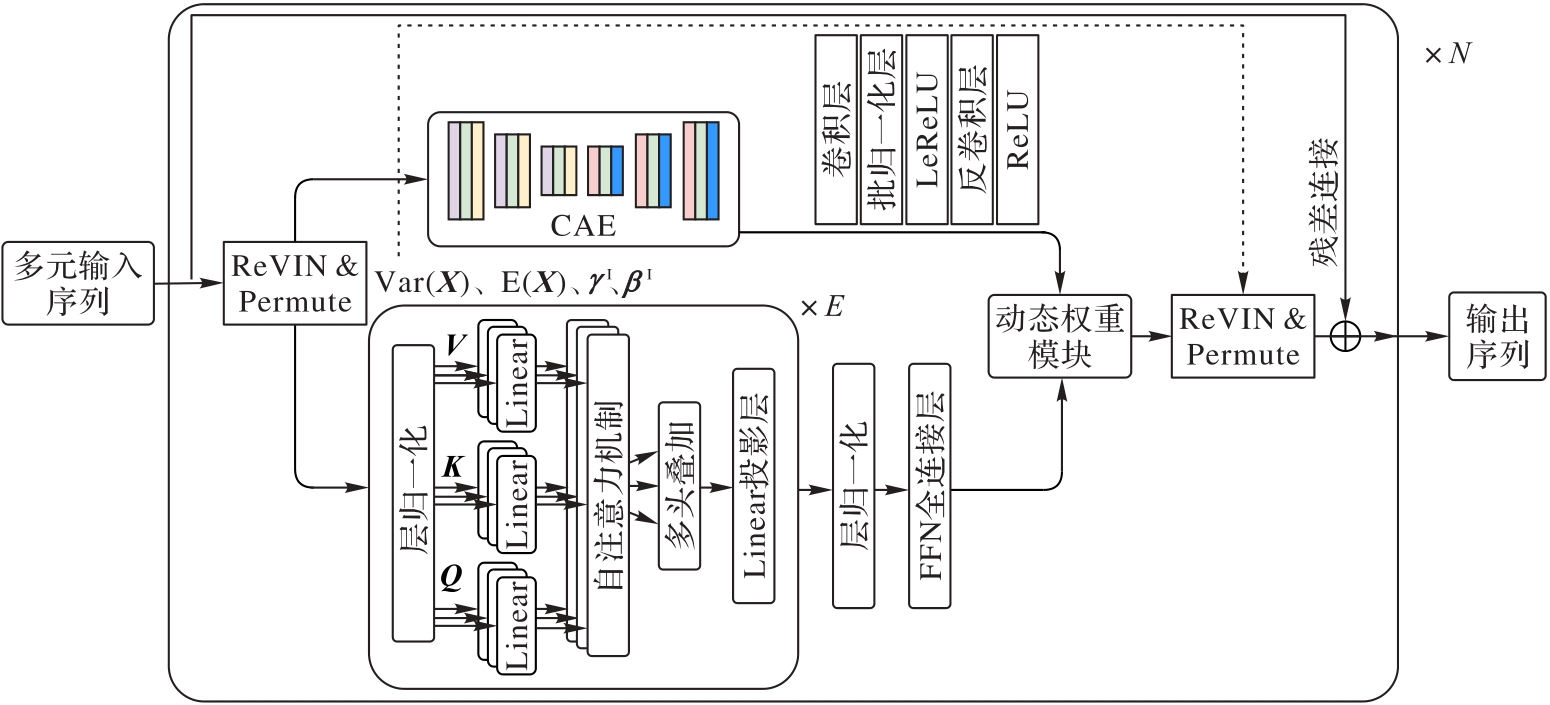
图1 模型的整体结构
Fig. 1 Overall structure of model

图2 AE压缩与CAE压缩的对比
Fig. 2 Comparison of AE compression and CAE compression
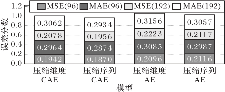
图3 转置实验结果
Fig. 3 Results of transposed experiments
| 方法 | Illness 36-36 | Illness 36-60 | ECL 96-96 | ECL 96-192 | ETTh1 96-96 | ETTh1 96-336 | ||||||
|---|---|---|---|---|---|---|---|---|---|---|---|---|
| MSE | MAE | MSE | MAE | MSE | MAE | MSE | MAE | MSE | MAE | MSE | MAE | |
| iTransformer | 2.268 | 0.972 | 2.274 | 0.979 | 0.148 | 0.260 | 0.178 | 0.269 | 0.392 | 0.410 | 0.490 | 0.462 |
| TimeMixer | 2.057 | 0.929 | 2.296 | 1.094 | 0.153 | 0.246 | 0.165 | 0.256 | 0.375 | 0.400 | 0.484 | 0.459 |
| TimesNet | 1.972 | 0.920 | 2.027 | 0.928 | 0.168 | 0.272 | 0.184 | 0.289 | 0.384 | 0.402 | 0.491 | 0.469 |
| DLinear | 1.963 | 0.963 | 2.368 | 1.096 | 0.140 | 0.237 | 0.169 | 0.267 | 0.375 | 0.399 | 0.489 | 0.457 |
| Autoformer | 3.103 | 1.287 | 2.700 | 1.125 | 0.201 | 0.317 | 0.222 | 0.334 | 0.477 | 0.478 | 0.566 | 0.525 |
| 本文方法 | 1.847 | 0.865 | 1.959 | 0.906 | 0.138 | 0.235 | 0.165 | 0.261 | 0.409 | 0.418 | 0.482 | 0.457 |
| 方法 | ETTm1 96-96 | ETTm1 96-336 | Exchange 96-96 | Exchange 96-336 | Weather 96-96 | Weather 96-336 | ||||||
| MSE | MAE | MSE | MAE | MSE | MAE | MSE | MAE | MSE | MAE | MSE | MAE | |
| iTransformer | 0.338 | 0.373 | 0.426 | 0.422 | 0.091 | 0.216 | 0.331 | 0.417 | 0.174 | 0.214 | 0.278 | 0.297 |
| TimeMixer | 0.320 | 0.356 | 0.390 | 0.405 | 0.089 | 0.211 | 0.339 | 0.420 | 0.163 | 0.210 | 0.251 | 0.289 |
| TimesNet | 0.338 | 0.375 | 0.410 | 0.411 | 0.107 | 0.234 | 0.367 | 0.448 | 0.172 | 0.220 | 0.280 | 0.306 |
| DLinear | 0.328 | 0.362 | 0.400 | 0.406 | 0.092 | 0.213 | 0.305 | 0.414 | 0.176 | 0.237 | 0.259 | 0.322 |
| Autoformer | 0.526 | 0.488 | 0.593 | 0.521 | 0.197 | 0.323 | 0.509 | 0.524 | 0.266 | 0.336 | 0.359 | 0.395 |
| 本文方法 | 0.327 | 0.363 | 0.418 | 0.422 | 0.088 | 0.208 | 0.277 | 0.303 | 0.161 | 0.208 | 0.272 | 0.297 |
表1 预测实验结果对比
Tab. 1 Forecasting experimental results
| 方法 | Illness 36-36 | Illness 36-60 | ECL 96-96 | ECL 96-192 | ETTh1 96-96 | ETTh1 96-336 | ||||||
|---|---|---|---|---|---|---|---|---|---|---|---|---|
| MSE | MAE | MSE | MAE | MSE | MAE | MSE | MAE | MSE | MAE | MSE | MAE | |
| iTransformer | 2.268 | 0.972 | 2.274 | 0.979 | 0.148 | 0.260 | 0.178 | 0.269 | 0.392 | 0.410 | 0.490 | 0.462 |
| TimeMixer | 2.057 | 0.929 | 2.296 | 1.094 | 0.153 | 0.246 | 0.165 | 0.256 | 0.375 | 0.400 | 0.484 | 0.459 |
| TimesNet | 1.972 | 0.920 | 2.027 | 0.928 | 0.168 | 0.272 | 0.184 | 0.289 | 0.384 | 0.402 | 0.491 | 0.469 |
| DLinear | 1.963 | 0.963 | 2.368 | 1.096 | 0.140 | 0.237 | 0.169 | 0.267 | 0.375 | 0.399 | 0.489 | 0.457 |
| Autoformer | 3.103 | 1.287 | 2.700 | 1.125 | 0.201 | 0.317 | 0.222 | 0.334 | 0.477 | 0.478 | 0.566 | 0.525 |
| 本文方法 | 1.847 | 0.865 | 1.959 | 0.906 | 0.138 | 0.235 | 0.165 | 0.261 | 0.409 | 0.418 | 0.482 | 0.457 |
| 方法 | ETTm1 96-96 | ETTm1 96-336 | Exchange 96-96 | Exchange 96-336 | Weather 96-96 | Weather 96-336 | ||||||
| MSE | MAE | MSE | MAE | MSE | MAE | MSE | MAE | MSE | MAE | MSE | MAE | |
| iTransformer | 0.338 | 0.373 | 0.426 | 0.422 | 0.091 | 0.216 | 0.331 | 0.417 | 0.174 | 0.214 | 0.278 | 0.297 |
| TimeMixer | 0.320 | 0.356 | 0.390 | 0.405 | 0.089 | 0.211 | 0.339 | 0.420 | 0.163 | 0.210 | 0.251 | 0.289 |
| TimesNet | 0.338 | 0.375 | 0.410 | 0.411 | 0.107 | 0.234 | 0.367 | 0.448 | 0.172 | 0.220 | 0.280 | 0.306 |
| DLinear | 0.328 | 0.362 | 0.400 | 0.406 | 0.092 | 0.213 | 0.305 | 0.414 | 0.176 | 0.237 | 0.259 | 0.322 |
| Autoformer | 0.526 | 0.488 | 0.593 | 0.521 | 0.197 | 0.323 | 0.509 | 0.524 | 0.266 | 0.336 | 0.359 | 0.395 |
| 本文方法 | 0.327 | 0.363 | 0.418 | 0.422 | 0.088 | 0.208 | 0.277 | 0.303 | 0.161 | 0.208 | 0.272 | 0.297 |

图4 汇率数据集预测长度96的实验结果可视化
Fig. 4 Visualization of experimental results on exchange rate dataset with forecasting length of 96
| 模型 | 参数量/106 | 计算量/GMAC |
|---|---|---|
| iTransformer | 3.256 | 1.250 |
| TimeMixer | 1.128 | 57.980 |
| TimesNet | 36.744 | 676.854 |
| DLinear | 0.018 | 0.005 |
| Autoformer | 5.822 | 21.153 |
| 本文方法 | 1.431 | 0.011 |
表2 模型复杂度
Tab. 2 Method complexity
| 模型 | 参数量/106 | 计算量/GMAC |
|---|---|---|
| iTransformer | 3.256 | 1.250 |
| TimeMixer | 1.128 | 57.980 |
| TimesNet | 36.744 | 676.854 |
| DLinear | 0.018 | 0.005 |
| Autoformer | 5.822 | 21.153 |
| 本文方法 | 1.431 | 0.011 |
| 方法 | ECL 96-96 | ECL 96-192 | ETTm1 96-96 | ETTm1 96-336 | Exchange 96-96 | Exchange 96-336 | Weather 96-96 | Weather 96-336 |
|---|---|---|---|---|---|---|---|---|
| iTransformer | 0.045 | 0.065 | 0.056 | 0.081 | 0.016 | 0.003 | 0.003 | 0.027 |
| TimeMixer | 0.022 | 0.574 | 0.124 | 0.036 | 0.621 | 0.004 | 0.434 | 0.021 |
| TimesNet | 0.171 | 0.005 | 0.024 | 0.060 | 0.007 | 0.002 | 0.001 | 0.025 |
| DLinear | 0.361 | 0.026 | 0.108 | 0.339 | 0.017 | 0.046 | 0.010 | 0.080 |
| Autoformer | 0.001 | 0.012 | 0.001 | 0.003 | 0.000 | 0.001 | 0.001 | 0.003 |
表3 本文方法与基线方法的t检验结果
Tab. 3 t-test results of proposed method and baseline methods
| 方法 | ECL 96-96 | ECL 96-192 | ETTm1 96-96 | ETTm1 96-336 | Exchange 96-96 | Exchange 96-336 | Weather 96-96 | Weather 96-336 |
|---|---|---|---|---|---|---|---|---|
| iTransformer | 0.045 | 0.065 | 0.056 | 0.081 | 0.016 | 0.003 | 0.003 | 0.027 |
| TimeMixer | 0.022 | 0.574 | 0.124 | 0.036 | 0.621 | 0.004 | 0.434 | 0.021 |
| TimesNet | 0.171 | 0.005 | 0.024 | 0.060 | 0.007 | 0.002 | 0.001 | 0.025 |
| DLinear | 0.361 | 0.026 | 0.108 | 0.339 | 0.017 | 0.046 | 0.010 | 0.080 |
| Autoformer | 0.001 | 0.012 | 0.001 | 0.003 | 0.000 | 0.001 | 0.001 | 0.003 |
| 方法 | MSL | PSM | SMAP | ||||||
|---|---|---|---|---|---|---|---|---|---|
| 精确率 | 召回率 | F1分数 | 精确率 | 召回率 | F1分数 | 精确率 | 召回率 | F1分数 | |
| OmniAnomaly | 89.02 | 86.37 | 87.67 | 88.39 | 74.46 | 80.83 | 92.49 | 61.99 | 74.21 |
| iTransformer | 87.65 | 70.37 | 78.07 | 98.10 | 93.09 | 95.53 | 90.69 | 53.36 | 67.19 |
| TimesNet | 89.54 | 75.36 | 81.84 | 98.51 | 96.31 | 97.40 | 90.01 | 55.06 | 68.33 |
| DLinear | 89.86 | 75.12 | 81.83 | 98.28 | 89.26 | 93.55 | 89.90 | 54.04 | 67.50 |
| Autoformer | 77.27 | 80.92 | 79.05 | 99.08 | 88.15 | 93.29 | 90.40 | 58.62 | 71.12 |
| 本文方法 | 83.86 | 81.35 | 82.58 | 96.43 | 96.81 | 96.62 | 87.40 | 56.10 | 68.33 |
| 方法 | SMD | SWAT | 平均F1分数 | ||||||
| 精确率 | 召回率 | F1分数 | 精确率 | 召回率 | F1分数 | ||||
| OmniAnomaly | 83.68 | 86.82 | 85.22 | 81.42 | 84.30 | 82.83 | 82.16 | ||
| iTransformer | 87.58 | 78.77 | 82.94 | 92.18 | 93.08 | 92.63 | 83.27 | ||
| TimesNet | 87.62 | 79.98 | 83.63 | 88.31 | 96.24 | 92.10 | 84.66 | ||
| DLinear | 83.62 | 71.52 | 77.10 | 80.91 | 95.30 | 87.52 | 81.50 | ||
| Autoformer | 78.44 | 65.10 | 71.15 | 89.85 | 95.81 | 92.74 | 81.47 | ||
| 本文方法 | 86.25 | 81.10 | 83.59 | 93.76 | 93.26 | 93.51 | 84.92 | ||
表4 不同模型在不同数据集上的异常检测结果 (%)
Tab. 4 Anomaly detection results of different models on different datasets
| 方法 | MSL | PSM | SMAP | ||||||
|---|---|---|---|---|---|---|---|---|---|
| 精确率 | 召回率 | F1分数 | 精确率 | 召回率 | F1分数 | 精确率 | 召回率 | F1分数 | |
| OmniAnomaly | 89.02 | 86.37 | 87.67 | 88.39 | 74.46 | 80.83 | 92.49 | 61.99 | 74.21 |
| iTransformer | 87.65 | 70.37 | 78.07 | 98.10 | 93.09 | 95.53 | 90.69 | 53.36 | 67.19 |
| TimesNet | 89.54 | 75.36 | 81.84 | 98.51 | 96.31 | 97.40 | 90.01 | 55.06 | 68.33 |
| DLinear | 89.86 | 75.12 | 81.83 | 98.28 | 89.26 | 93.55 | 89.90 | 54.04 | 67.50 |
| Autoformer | 77.27 | 80.92 | 79.05 | 99.08 | 88.15 | 93.29 | 90.40 | 58.62 | 71.12 |
| 本文方法 | 83.86 | 81.35 | 82.58 | 96.43 | 96.81 | 96.62 | 87.40 | 56.10 | 68.33 |
| 方法 | SMD | SWAT | 平均F1分数 | ||||||
| 精确率 | 召回率 | F1分数 | 精确率 | 召回率 | F1分数 | ||||
| OmniAnomaly | 83.68 | 86.82 | 85.22 | 81.42 | 84.30 | 82.83 | 82.16 | ||
| iTransformer | 87.58 | 78.77 | 82.94 | 92.18 | 93.08 | 92.63 | 83.27 | ||
| TimesNet | 87.62 | 79.98 | 83.63 | 88.31 | 96.24 | 92.10 | 84.66 | ||
| DLinear | 83.62 | 71.52 | 77.10 | 80.91 | 95.30 | 87.52 | 81.50 | ||
| Autoformer | 78.44 | 65.10 | 71.15 | 89.85 | 95.81 | 92.74 | 81.47 | ||
| 本文方法 | 86.25 | 81.10 | 83.59 | 93.76 | 93.26 | 93.51 | 84.92 | ||
| 方法 | ill_national 36-36 | ill_national 36-60 | ECL 96-96 | ECL 96-192 | ETTh1 96-96 | ETTh1 96-336 | ||||||
|---|---|---|---|---|---|---|---|---|---|---|---|---|
| MSE | MAE | MSE | MAE | MSE | MAE | MSE | MAE | MSE | MAE | MSE | MAE | |
| 去除自注意力机制 | 2.403 | 1.001 | 2.176 | 0.935 | 0.147 | 0.244 | 0.173 | 0.264 | 0.520 | 0.484 | 0.522 | 0.477 |
| 去除归一化 | 2.200 | 0.965 | 2.170 | 0.942 | 0.156 | 0.255 | 0.163 | 0.258 | 0.471 | 0.459 | 0.503 | 0.472 |
| 去除卷积自编码器 | 2.428 | 0.983 | 2.633 | 1.045 | 0.156 | 0.260 | 0.158 | 0.253 | 0.395 | 0.409 | 0.488 | 0.461 |
| 替换自编码器 | 2.203 | 0.919 | 2.165 | 0.957 | 0.140 | 0.237 | 0.178 | 0.283 | 0.424 | 0.439 | 0.483 | 0.458 |
| 去除动态权重 | 2.549 | 1.016 | 2.492 | 1.047 | 0.180 | 0.289 | 0.170 | 0.264 | 0.395 | 0.410 | 0.504 | 0.473 |
| 本文方法 | 1.847 | 0.865 | 1.959 | 0.906 | 0.138 | 0.235 | 0.155 | 0.251 | 0.409 | 0.418 | 0.486 | 0.460 |
| 方法 | ETTm1 96-96 | ETTm1 96-336 | Exchange 96-96 | Exchange 96-336 | Weather 96-96 | Weather 96-336 | ||||||
| MSE | MAE | MSE | MAE | MSE | MAE | MSE | MAE | MSE | MAE | MSE | MAE | |
| 去除自注意力机制 | 0.332 | 0.363 | 0.447 | 0.426 | 0.095 | 0.219 | 0.336 | 0.420 | 0.170 | 0.216 | 0.275 | 0.300 |
| 去除归一化 | 0.337 | 0.371 | 0.443 | 0.433 | 0.095 | 0.216 | 0.327 | 0.414 | 0.166 | 0.213 | 0.281 | 0.304 |
| 去除卷积自编码器 | 0.333 | 0.368 | 0.446 | 0.432 | 0.096 | 0.217 | 0.326 | 0.414 | 0.162 | 0.208 | 0.265 | 0.292 |
| 替换自编码器 | 0.336 | 0.369 | 0.427 | 0.422 | 0.087 | 0.208 | 0.332 | 0.417 | 0.164 | 0.215 | 0.269 | 0.293 |
| 去除动态权重 | 0.367 | 0.391 | 0.419 | 0.416 | 0.088 | 0.211 | 0.343 | 0.425 | 0.166 | 0.215 | 0.283 | 0.307 |
| 本文方法 | 0.327 | 0.364 | 0.418 | 0.422 | 0.088 | 0.209 | 0.277 | 0.303 | 0.161 | 0.208 | 0.272 | 0.297 |
表5 消融实验结果
Tab. 5 Results of ablation experiments
| 方法 | ill_national 36-36 | ill_national 36-60 | ECL 96-96 | ECL 96-192 | ETTh1 96-96 | ETTh1 96-336 | ||||||
|---|---|---|---|---|---|---|---|---|---|---|---|---|
| MSE | MAE | MSE | MAE | MSE | MAE | MSE | MAE | MSE | MAE | MSE | MAE | |
| 去除自注意力机制 | 2.403 | 1.001 | 2.176 | 0.935 | 0.147 | 0.244 | 0.173 | 0.264 | 0.520 | 0.484 | 0.522 | 0.477 |
| 去除归一化 | 2.200 | 0.965 | 2.170 | 0.942 | 0.156 | 0.255 | 0.163 | 0.258 | 0.471 | 0.459 | 0.503 | 0.472 |
| 去除卷积自编码器 | 2.428 | 0.983 | 2.633 | 1.045 | 0.156 | 0.260 | 0.158 | 0.253 | 0.395 | 0.409 | 0.488 | 0.461 |
| 替换自编码器 | 2.203 | 0.919 | 2.165 | 0.957 | 0.140 | 0.237 | 0.178 | 0.283 | 0.424 | 0.439 | 0.483 | 0.458 |
| 去除动态权重 | 2.549 | 1.016 | 2.492 | 1.047 | 0.180 | 0.289 | 0.170 | 0.264 | 0.395 | 0.410 | 0.504 | 0.473 |
| 本文方法 | 1.847 | 0.865 | 1.959 | 0.906 | 0.138 | 0.235 | 0.155 | 0.251 | 0.409 | 0.418 | 0.486 | 0.460 |
| 方法 | ETTm1 96-96 | ETTm1 96-336 | Exchange 96-96 | Exchange 96-336 | Weather 96-96 | Weather 96-336 | ||||||
| MSE | MAE | MSE | MAE | MSE | MAE | MSE | MAE | MSE | MAE | MSE | MAE | |
| 去除自注意力机制 | 0.332 | 0.363 | 0.447 | 0.426 | 0.095 | 0.219 | 0.336 | 0.420 | 0.170 | 0.216 | 0.275 | 0.300 |
| 去除归一化 | 0.337 | 0.371 | 0.443 | 0.433 | 0.095 | 0.216 | 0.327 | 0.414 | 0.166 | 0.213 | 0.281 | 0.304 |
| 去除卷积自编码器 | 0.333 | 0.368 | 0.446 | 0.432 | 0.096 | 0.217 | 0.326 | 0.414 | 0.162 | 0.208 | 0.265 | 0.292 |
| 替换自编码器 | 0.336 | 0.369 | 0.427 | 0.422 | 0.087 | 0.208 | 0.332 | 0.417 | 0.164 | 0.215 | 0.269 | 0.293 |
| 去除动态权重 | 0.367 | 0.391 | 0.419 | 0.416 | 0.088 | 0.211 | 0.343 | 0.425 | 0.166 | 0.215 | 0.283 | 0.307 |
| 本文方法 | 0.327 | 0.364 | 0.418 | 0.422 | 0.088 | 0.209 | 0.277 | 0.303 | 0.161 | 0.208 | 0.272 | 0.297 |
| 方法 | 96-96 | 96-192 | ||
|---|---|---|---|---|
| MSE | MAE | MSE | MAE | |
| iTransformer | 0.276 | 0.666 | 0.336 | 1.143 |
| TimeMixer | 0.283 | 0.671 | 0.342 | 0.659 |
| DLinear | 0.375 | 0.650 | 0.362 | 0.594 |
| Autoformer | 0.445 | 1.103 | 0.532 | 1.311 |
| 本文方法 | 0.250 | 0.612 | 0.308 | 0.688 |
表6 白洋淀水质环境监测数据预测的实验结果对比
Tab. 6 Comparison of experimental results of water quality monitoring data forecasting in Baiyangdian Lake
| 方法 | 96-96 | 96-192 | ||
|---|---|---|---|---|
| MSE | MAE | MSE | MAE | |
| iTransformer | 0.276 | 0.666 | 0.336 | 1.143 |
| TimeMixer | 0.283 | 0.671 | 0.342 | 0.659 |
| DLinear | 0.375 | 0.650 | 0.362 | 0.594 |
| Autoformer | 0.445 | 1.103 | 0.532 | 1.311 |
| 本文方法 | 0.250 | 0.612 | 0.308 | 0.688 |
| [1] | Wu H, Xu J, Wang J, et al. Autoformer: decomposition Transformers with auto-correlation for long-term series forecasting[C]// NeurIPS 2021. Red Hook: Curran Associates Inc., 2021: 22419-22430. |
| [2] | Franceschi J Y, Dieuveut A, Jaggi M. Unsupervised scalable representation learning for multivariate time series[C]// NeurIPS 2019. Red Hook: Curran Associates Inc., 2019: 7650-7661. |
| [3] | Lai K H, Zha D, Xu J, et al. Revisiting time series outlier detection: definitions and benchmarks[EB/OL]. (2021) [2024-06-10].. |
| [4] | Friedman M. The interpolation of time series by related series[J]. Journal of the American Statistical Association, 1962, 57(300): 729-757. |
| [5] | Box G E P, Jenkins G M, Reinsel G C, et al. Time series analysis: forecasting and control[M]. 5th ed. Hoboken, NJ: John Wiley & Sons, Inc., 2015: 1-10. |
| [6] | Dietterich T G. Machine learning for sequential data: a review[C]// SSPR/SPR 2002, LNCS 2396. Berlin: Springer, 2002: 15-30. |
| [7] | Ashenfelter O. Estimating the effect of training programs on earnings[J]. The Review of Economics and Statistics, 1978, 60(4): 47-57. |
| [8] | Elman J L. Finding structure in time[J]. Cognitive Science, 1990, 14(2): 179-211. |
| [9] | Liu X, Ren J S J, Liu C, et al. Deep convolutional neural network for image deconvolution[C]// NeurIPS 2014 — Volume 1. Cambridge: MIT Press, 2014: 1790-1798. |
| [10] | Bai S, Kolter J Z, Koltun V. An empirical evaluation of generic convolutional and recurrent networks for sequence modeling[PP/OL]. V2. arXiv (2018-04-19) [2024-06-05].. |
| [11] | Wu H, Hu T, Liu Y, et al. TimesNet: temporal 2D-variation modeling for general time series analysis[PP/OL]. V2. arXiv (2023-04-12) [2024-06-08].. |
| [12] | Wang S, Wu H, Shi X, et al. TimeMixer: decomposable multiscale mixing for time series forecasting[PP/OL]. arXiv (2024-05-23) [2024-06-08].. |
| [13] | Hinton G E, Salakhutdinov R R. Reducing the dimensionality of data with neural networks[J]. Science, 2006, 313(5786): 504-507. |
| [14] | Hinton G E, Sejnowski T J. Learning and relearning in Boltzmann machines[M]// Jordan M I, Sejnowski T J. Graphical models: foundations of neural computation. Cambridge: MIT Press, 2001: 45-76. |
| [15] | 李永飞,李铭洋,常鑫,等. 基于可解释性深度学习的物联网水质监测数据异常检测[J]. 计算机工程, 2024, 50(6): 179-187. |
| Li Yongfei, Li Mingyang, Chang Xin, et al. Anomaly detection of IoT water quality monitoring data based on explainable deep learning[J]. Computer Engineering, 2024, 50(6): 179-187. | |
| [16] | Yao Y, Ma J, Ye Y. Regularizing autoencoders with wavelet transform for sequence anomaly detection[J]. Pattern Recognition, 2023, 134: No.109084. |
| [17] | Kingma D P, Welling M. Auto-encoding variational Bayes[PP/OL]. V11. arXiv (2022-12-10) [2024-06-06].. |
| [18] | An J, Cho S. Variational autoencoder based anomaly detection using reconstruction probability[R/OL]. (2015-12-27) [2024-06-09].. |
| [19] | Vaswani A, Shazeer N, Parmar N, et al. Attention is all you need[C]// NeurIPS 2017. Red Hook: Curran Associates Inc., 2017: 6000-6010. |
| [20] | Zeng A, Chen M, Zhang L, et al. Are Transformers effective for time series forecasting?[J]. Proceedings of the AAAI Conference on Artificial Intelligence, 2023, 37(9): 11121-11128. |
| [21] | Liu Y, Hu T, Zhang H, et al. iTransformer: inverted Transformers are effective for time series forecasting[PP/OL]. V4. arXiv (2024-03-14) [2024-06-09].. |
| [22] | Zhou H, Zhang S, Peng J, et al. Informer: beyond efficient Transformer for long sequence time-series forecasting[J]. Proceedings of the AAAI Conference on Artificial Intelligence, 2021, 35(12): 11106-11115. |
| [23] | Tuli S, Casale G, Jennings N R. TranAD: deep Transformer networks for anomaly detection in multivariate time series data[J]. Proceedings of the VLDB Endowment, 2022, 15(6): 1201-1214. |
| [24] | Goodfellow I, Pouget-Abadie J, Mirza M, et al. Generative adversarial nets[C]// NeurIPS 2014 — Volume 2. Cambridge: MIT Press, 2014: 2672-2680. |
| [25] | Nie Y, Nguyen N H, Sinthong P, et al. A time series is worth 64 words: long-term forecasting with Transformers[PP/OL]. V2. arXiv (2023-03-04) [2024-06-09].. |
| [26] | Liu Y, Wu H, Wang J, et al. Non-stationary Transformers: exploring the stationarity in time series forecasting[C]// NeurIPS 2022. Red Hook: Curran Associates Inc., 2022: 9881-9893. |
| [27] | Xu J, Wu H, Wang J, et al. Anomaly Transformer: time series anomaly detection with association discrepancy[PP/OL]. V5. arXiv (2022-06-29) [2024-06-08].. |
| [28] | Zhang Y, Yan J. Crossformer: Transformer utilizing cross-dimension dependency for multivariate time series forecasting[EB/OL]. (2023-03-02) [2024-06-07].. |
| [29] | Darban Z Z, Webb G I, Pan S, et al. Deep learning for time series anomaly detection: a survey[J]. ACM Computing Surveys, 2025, 57(1): No.15. |
| [30] | Zhang Y. A better autoencoder for image: convolutional autoencoder[EB/OL]. (2019-01-02) [2024-06-06].. |
| [31] | Nair V, Hinton G E. Rectified linear units improve restricted Boltzmann machines[C]// ICML 2010. Madison, WI: Omnipress, 2010: 807-814. |
| [32] | Maas A L, Hannun A Y, Ng A Y. Rectifier nonlinearities improve neural network acoustic models[EB/OL]. (2013) [2024-06-06].. |
| [33] | Ba J L, Kiros J R, Hinton G E. Layer normalization[PP/OL]. arXiv (2016-07-21) [2024-06-05].. |
| [34] | Ioffe S, Szegedy C. Batch normalization: accelerating deep network training by reducing internal covariate shift[J]. Proceedings of Machine Learning Research, 2015, 37: 448-456. |
| [35] | Kim T, Kim J, Tae Y, et al. Reversible instance normalization for accurate time-series forecasting against distribution shift[EB/OL]. (2023-02-14) [2024-06-07].. |
| [36] | Trindade A. ElectricityLoadDiagrams20112014[DS/OL]. (2015) [2024-06-10].. |
| [37] | Centers for Disease Control and Prevention. National, regional, and state level outpatient illness and viral surveillance[EB/OL]. [2024-06-10].. |
| [38] | Lai G, Chang W C, Yang Y, et al. Modeling long- and short-term temporal patterns with deep neural networks[C]// SIGIR 2018. New York: ACM, 2018: 95-104. |
| [39] | Su Y, Zhao Y, Niu C, et al. Robust anomaly detection for multivariate time series through stochastic recurrent neural network[C]// KDD 2019. New York: ACM, 2019: 2828-2837. |
| [40] | Hundman K, Constantinou V, Laporte C, et al. Detecting spacecraft anomalies using LSTMs and nonparametric dynamic thresholding[C]// KDD 2018. New York: ACM, 2018: 387-395. |
| [41] | Su J, Vargas D V, Sakurai K. One pixel attack for fooling deep neural networks[J]. IEEE Transactions on Evolutionary Computation, 2019, 23(5): 828-841. |
| [42] | Mathur A P, Tippenhauer N O. SWaT: a water treatment testbed for research and training on ICS security[C]// CySWater 2016. Piscataway: IEEE, 2016: 31-36. |
| [43] | Abdulaal A, Lancewicki T. Real-time synchronization in neural networks for multivariate time series anomaly detection[C]// ICASSP 2021. Piscataway: IEEE, 2021: 3570-3574. |
| [1] | 李栋, 赵苡积, 丁海燕, 武浩. 基于软白化的无负样本自监督学习时序预测框架[J]. 《计算机应用》唯一官方网站, 2026, 46(8): 2457-2466. |
| [2] | 任志强, 陈学斌, 屈昌盛. 面向联邦学习中拜占庭攻击的主动防御框架[J]. 《计算机应用》唯一官方网站, 2026, 46(7): 2196-2207. |
| [3] | 杜秀丽, 高星, 张校毓, 潘成胜, 邹启杰. 基于密集时空可变形注意力的视频快照压缩成像重建方法[J]. 《计算机应用》唯一官方网站, 2026, 46(7): 2288-2296. |
| [4] | 陈坚伟, 陆佳炜, 王琪冰, 赵梦珂. 基于动态时空编码器的电梯多元时间序列异常检测方法[J]. 《计算机应用》唯一官方网站, 2026, 46(7): 2364-2372. |
| [5] | 何运平, 王雷春, 宋芮芮, 卢祥凤, 魏金香, 刘小萌. 基于对比不变性和强化特定性的双通道多模态情感分析模型[J]. 《计算机应用》唯一官方网站, 2026, 46(6): 1767-1775. |
| [6] | 王倩飞, 李旸, 李德玉, 王素格. 基于大语言模型的双通道特征融合表示的短文本聚类方法[J]. 《计算机应用》唯一官方网站, 2026, 46(5): 1441-1449. |
| [7] | 宋芮芮, 王雷春, 何运平, 魏金香, 卢祥凤, 刘小萌. 基于混合自注意力和差异归一化的长时间序列预测[J]. 《计算机应用》唯一官方网站, 2026, 46(5): 1499-1506. |
| [8] | 谢斌红, 朱二丹, 张睿. 基于外观-运动协同建模的视频异常检测[J]. 《计算机应用》唯一官方网站, 2026, 46(5): 1551-1559. |
| [9] | 索逸凡, 刘松华, 郝秋智. 基于高阶特征聚合的时间序列异常检测方法[J]. 《计算机应用》唯一官方网站, 2026, 46(4): 1131-1138. |
| [10] | 尹春勇, 张不凡. 基于多尺度的多变量时间序列异常检测模型[J]. 《计算机应用》唯一官方网站, 2026, 46(3): 790-797. |
| [11] | 董莉梅, 李雁姿, 李家印, 许力. 基于邻域增强的无监督图异常检测[J]. 《计算机应用》唯一官方网站, 2026, 46(2): 458-466. |
| [12] | 韩锋, 卜永丰, 梁浩翔, 黄舒雯, 张朝阳, 孙士杰. 基于多层次时空交互依赖的车辆轨迹异常检测[J]. 《计算机应用》唯一官方网站, 2026, 46(2): 604-612. |
| [13] | 罗虎, 张明书. 基于跨模态注意力机制与对比学习的谣言检测方法[J]. 《计算机应用》唯一官方网站, 2026, 46(2): 361-367. |
| [14] | 钟琪, 张淑芬, 张镇博, 菅银龙, 景忠瑞. 面向联邦学习的投毒攻击检测与防御机制[J]. 《计算机应用》唯一官方网站, 2026, 46(2): 445-457. |
| [15] | 魏金香, 王雷春, 卢祥凤, 宋芮芮, 何运平, 刘小萌. 融合时空感知与自监督转换器的交通流预测模型[J]. 《计算机应用》唯一官方网站, 2026, 46(10): 3171-3179. |
| 阅读次数 | ||||||
|
全文 |
|
|||||
|
摘要 |
|
|||||
