


《计算机应用》唯一官方网站 ›› 2026, Vol. 46 ›› Issue (8): 2457-2466.DOI: 10.11772/j.issn.1001-9081.2025070823
李栋, 赵苡积, 丁海燕( ), 武浩
), 武浩
收稿日期:2025-07-23
修回日期:2025-10-13
接受日期:2025-10-14
发布日期:2025-11-05
出版日期:2026-08-10
通讯作者:
丁海燕
作者简介:李栋(1999—),男,上海人,硕士研究生,主要研究方向:时空数据挖掘、网络表征学习基金资助:
Dong LI, Yiji ZHAO, Haiyan DING(), Hao WU
Received:2025-07-23
Revised:2025-10-13
Accepted:2025-10-14
Online:2025-11-05
Published:2026-08-10
Contact:
Haiyan DING
About author:LI Dong, born in 1999, M. S. candidate. His research interests include spatio-temporal data mining, network representation learning.Supported by:摘要:
针对现有的自监督学习方法在时序领域存在的依赖负样本对以及数据增强可能破坏时序结构等问题,提出一种基于软白化的无负样本自监督学习时序预测框架(SWTF)。该框架旨在无需负样本即可学习到信息密集且具备预测能力的序列表征。它的核心方法包含两个协同优化目标:一是时序软白化(TSW)损失,即减少表征维度间的冗余并维持表征的方差学习紧凑且信息丰富的表征,从而避免对负样本对和表征不变性约束的依赖;二是去噪重构任务,即通过有针对性的任务设计,引导模型关注并编码具有预测性的时序特征。为了实现上述两个目标的联合优化,构建一个孪生编码器,利用并行多尺度卷积网络高效捕捉从微观的局部周期性到宏观的长程依赖关系。在电力、气象和交通等多个基准数据集上,相较于CoST和PDF(Periodicity Decoupling Framework)等主流时序预测基线,SWTF的平均绝对误差(MAE)降幅约为19.6% (13.4%~26.4%),证实了SWTF在学习鲁棒性和预测性较强的时间序列表征方面的有效性。
中图分类号:
李栋, 赵苡积, 丁海燕, 武浩. 基于软白化的无负样本自监督学习时序预测框架[J]. 计算机应用, 2026, 46(8): 2457-2466.
Dong LI, Yiji ZHAO, Haiyan DING, Hao WU. Soft whitening inspired non-contrastive SSL framework for time-series forecasting[J]. Journal of Computer Applications, 2026, 46(8): 2457-2466.
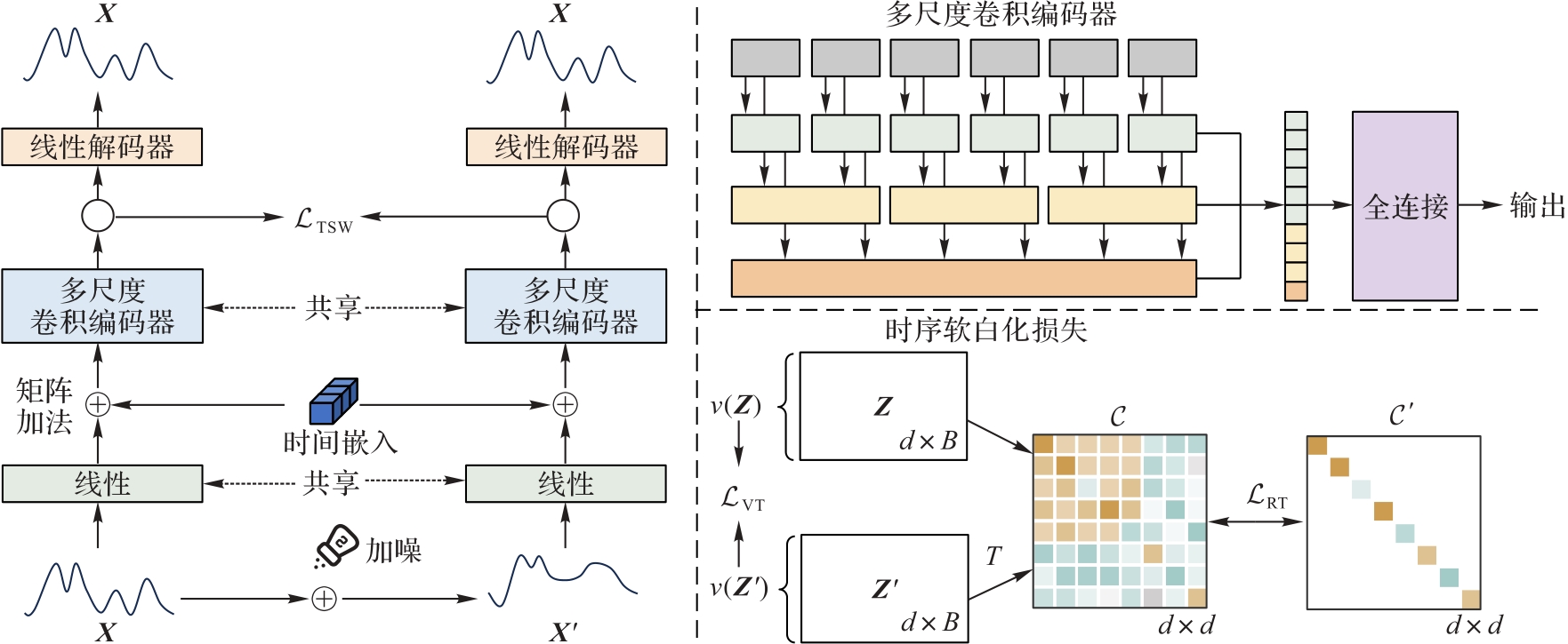
图1 SWTF的整体架构
Fig. 1 Overall architecture of SWTF
| 数据集 | 领域 | 采样间隔/min | 特征维度 | 样本数 |
|---|---|---|---|---|
| ETTh1 | 电力 | 60 | 7 | 17 420 |
| ETTh2 | 电力 | 60 | 7 | 17 420 |
| ETTm1 | 电力 | 15 | 7 | 69 680 |
| Traffic | 交通 | 60 | 862 | 17 544 |
| Weather | 天气 | 60 | 12 | 35 065 |
| PEMS08 | 交通 | 5 | 170 | 17 856 |
| Solar | 能源 | 10 | 137 | 52 559 |
表1 实验所用数据集的统计信息
Tab. 1 Statistics of datasets used in experiments
| 数据集 | 领域 | 采样间隔/min | 特征维度 | 样本数 |
|---|---|---|---|---|
| ETTh1 | 电力 | 60 | 7 | 17 420 |
| ETTh2 | 电力 | 60 | 7 | 17 420 |
| ETTm1 | 电力 | 15 | 7 | 69 680 |
| Traffic | 交通 | 60 | 862 | 17 544 |
| Weather | 天气 | 60 | 12 | 35 065 |
| PEMS08 | 交通 | 5 | 170 | 17 856 |
| Solar | 能源 | 10 | 137 | 52 559 |
| 数据集 | L | TimesURL(U) | TS2Vec(U) | SoftCLT(U) | CoST(U) | T-Rep(U) | PDF(S) | SWTF(U) | |||||||
|---|---|---|---|---|---|---|---|---|---|---|---|---|---|---|---|
| MSE | MAE | MSE | MAE | MSE | MAE | MSE | MAE | MSE | MAE | MSE | MAE | MSE | MAE | ||
| ETTh1 | 48 | 0.068 5 | 0.198 5 | 0.064 5 | 0.195 2 | 0.059 7 | 0.186 0 | 0.063 3 | 0.191 9 | 0.060 5 | 0.187 6 | 0.051 3 | 0.173 6 | ||
| 168 | 0.134 4 | 0.282 2 | 0.111 6 | 0.254 4 | 0.122 1 | 0.270 2 | 0.094 2 | 0.115 9 | 0.263 5 | 0.232 9 | 0.077 7 | 0.212 2 | |||
| 336 | 0.152 3 | 0.305 4 | 0.126 8 | 0.275 0 | 0.136 9 | 0.290 9 | 0.113 4 | 0.140 9 | 0.296 7 | 0.259 3 | 0.078 4 | 0.219 7 | |||
| 720 | 0.184 8 | 0.349 5 | 0.150 6 | 0.310 7 | 0.198 8 | 0.368 9 | 0.216 1 | 0.392 6 | 0.196 4 | 0.369 9 | 0.119 8 | 0.274 8 | |||
| ETTh2 | 48 | 0.186 5 | 0.331 6 | 0.138 6 | 0.289 3 | 0.127 3 | 0.278 5 | 0.107 2 | 0.118 0 | 0.259 9 | 0.250 6 | 0.099 1 | 0.245 9 | ||
| 168 | 0.252 8 | 0.396 7 | 0.211 1 | 0.359 6 | 0.194 4 | 0.345 8 | 0.310 8 | 0.187 4 | 0.337 5 | 0.181 8 | 0.330 9 | 0.158 6 | |||
| 336 | 0.302 0 | 0.436 5 | 0.259 9 | 0.404 5 | 0.243 9 | 0.391 5 | 0.242 4 | 0.392 6 | 0.212 5 | 0.365 7 | 0.192 5 | 0.352 7 | |||
| 720 | 0.360 7 | 0.482 4 | 0.292 4 | 0.436 7 | 0.272 6 | 0.421 4 | 0.292 5 | 0.439 5 | 0.318 4 | 0.462 2 | 0.234 4 | 0.395 1 | |||
| ETTm1 | 48 | 0.029 6 | 0.129 8 | 0.030 4 | 0.133 9 | 0.030 1 | 0.135 9 | 0.121 9 | 0.031 8 | 0.134 0 | 0.033 8 | 0.139 8 | 0.026 1 | ||
| 96 | 0.046 6 | 0.166 7 | 0.046 6 | 0.166 2 | 0.042 3 | 0.159 0 | 0.094 9 | 0.242 6 | 0.061 8 | 0.195 3 | 0.035 2 | 0.143 2 | |||
| 288 | 0.103 5 | 0.250 8 | 0.106 2 | 0.249 5 | 0.094 1 | 0.230 7 | 0.177 1 | 0.345 6 | 0.150 9 | 0.315 9 | 0.063 4 | 0.188 2 | |||
| 672 | 0.155 3 | 0.315 6 | 0.162 0 | 0.316 6 | 0.150 9 | 0.298 7 | 0.240 8 | 0.413 8 | 0.234 3 | 0.407 0 | 0.092 2 | 0.226 6 | |||
| Traffic | 48 | 0.640 8 | 0.584 8 | 0.457 1 | 0.497 8 | 0.484 8 | 0.509 9 | 0.427 3 | 0.491 8 | 0.519 4 | 0.496 5 | 0.198 3 | 0.291 1 | ||
| 168 | 0.660 6 | 0.601 8 | 0.503 7 | 0.529 7 | 0.511 0 | 0.528 2 | 0.421 9 | 0.490 0 | 0.529 6 | 0.517 6 | 0.218 5 | 0.302 4 | |||
| 336 | 0.682 0 | 0.615 6 | 0.502 5 | 0.529 8 | 0.517 9 | 0.532 9 | 0.429 7 | 0.497 9 | 0.526 3 | 0.523 1 | 0.237 5 | 0.316 7 | |||
| 720 | 0.668 5 | 0.606 7 | 0.499 7 | 0.524 9 | 0.519 0 | 0.531 7 | 0.434 1 | 0.496 7 | 0.545 1 | 0.537 7 | 0.280 4 | 0.348 8 | |||
| Weather | 48 | 0.152 7 | 0.276 3 | 0.153 0 | 0.274 0 | 0.157 1 | 0.277 6 | 0.143 0 | 0.198 2 | 0.308 7 | 0.264 2 | 0.133 0 | 0.254 0 | ||
| 168 | 0.242 9 | 0.359 0 | 0.242 4 | 0.359 1 | 0.259 1 | 0.372 6 | 0.227 3 | 0.281 2 | 0.378 8 | 0.346 5 | 0.204 7 | 0.328 0 | |||
| 336 | 0.280 7 | 0.392 3 | 0.274 4 | 0.390 1 | 0.297 5 | 0.407 2 | 0.353 3 | 0.426 6 | 0.269 6 | 0.384 8 | 0.258 4 | 0.373 3 | |||
| 720 | 0.302 6 | 0.413 0 | 0.277 9 | 0.398 2 | 0.303 4 | 0.415 6 | 0.529 3 | 0.538 1 | 0.358 4 | 0.456 5 | 0.358 6 | 0.457 2 | |||
| PEMS08 | 12 | 0.079 7 | 0.198 7 | 0.074 2 | 0.190 9 | 0.076 0 | 0.192 6 | 0.085 8 | 0.197 8 | 0.084 4 | 0.200 1 | 0.070 5 | 0.188 7 | ||
| 24 | 0.124 9 | 0.247 2 | 0.111 3 | 0.233 1 | 0.114 0 | 0.234 9 | 0.146 3 | 0.256 4 | 0.126 4 | 0.242 6 | 0.092 6 | 0.213 5 | |||
| 48 | 0.168 8 | 0.305 8 | 0.143 4 | 0.148 9 | 0.281 2 | 0.225 5 | 0.340 3 | 0.163 0 | 0.293 1 | 0.285 6 | 0.119 0 | 0.244 8 | |||
| 96 | 0.232 6 | 0.366 5 | 0.177 5 | 0.309 6 | 0.193 9 | 0.327 0 | 0.257 1 | 0.379 9 | 0.203 8 | 0.337 5 | 0.148 7 | 0.265 8 | |||
| Solar | 48 | 0.320 2 | 0.361 9 | 0.199 8 | 0.281 8 | 0.247 5 | 0.318 9 | 0.171 2 | 0.253 4 | 0.329 0 | 0.152 3 | 0.242 4 | 0.208 1 | ||
| 168 | 0.305 1 | 0.338 1 | 0.236 3 | 0.292 1 | 0.259 5 | 0.310 3 | 0.199 0 | 0.267 3 | 0.322 0 | 0.183 2 | 0.261 1 | 0.226 8 | |||
| 336 | 0.359 6 | 0.377 4 | 0.282 7 | 0.324 3 | 0.314 6 | 0.347 4 | 0.239 7 | 0.308 8 | 0.353 0 | 0.206 1 | 0.275 2 | 0.250 6 | |||
| 720 | 0.369 2 | 0.380 8 | 0.292 1 | 0.326 9 | 0.319 8 | 0.347 9 | 0.246 7 | 0.314 9 | 0.354 0 | 0.209 1 | 0.278 2 | 0.252 5 | |||
| 平均 | 0.270 3 | 0.359 7 | 0.218 7 | 0.325 6 | 0.228 6 | 0.333 0 | 0.199 7 | 0.254 5 | 0.352 5 | 0.155 6 | 0.264 2 | ||||
表2 各模型的单变量预测性能对比
Tab. 2 Comparison of univariate prediction performance of various models
| 数据集 | L | TimesURL(U) | TS2Vec(U) | SoftCLT(U) | CoST(U) | T-Rep(U) | PDF(S) | SWTF(U) | |||||||
|---|---|---|---|---|---|---|---|---|---|---|---|---|---|---|---|
| MSE | MAE | MSE | MAE | MSE | MAE | MSE | MAE | MSE | MAE | MSE | MAE | MSE | MAE | ||
| ETTh1 | 48 | 0.068 5 | 0.198 5 | 0.064 5 | 0.195 2 | 0.059 7 | 0.186 0 | 0.063 3 | 0.191 9 | 0.060 5 | 0.187 6 | 0.051 3 | 0.173 6 | ||
| 168 | 0.134 4 | 0.282 2 | 0.111 6 | 0.254 4 | 0.122 1 | 0.270 2 | 0.094 2 | 0.115 9 | 0.263 5 | 0.232 9 | 0.077 7 | 0.212 2 | |||
| 336 | 0.152 3 | 0.305 4 | 0.126 8 | 0.275 0 | 0.136 9 | 0.290 9 | 0.113 4 | 0.140 9 | 0.296 7 | 0.259 3 | 0.078 4 | 0.219 7 | |||
| 720 | 0.184 8 | 0.349 5 | 0.150 6 | 0.310 7 | 0.198 8 | 0.368 9 | 0.216 1 | 0.392 6 | 0.196 4 | 0.369 9 | 0.119 8 | 0.274 8 | |||
| ETTh2 | 48 | 0.186 5 | 0.331 6 | 0.138 6 | 0.289 3 | 0.127 3 | 0.278 5 | 0.107 2 | 0.118 0 | 0.259 9 | 0.250 6 | 0.099 1 | 0.245 9 | ||
| 168 | 0.252 8 | 0.396 7 | 0.211 1 | 0.359 6 | 0.194 4 | 0.345 8 | 0.310 8 | 0.187 4 | 0.337 5 | 0.181 8 | 0.330 9 | 0.158 6 | |||
| 336 | 0.302 0 | 0.436 5 | 0.259 9 | 0.404 5 | 0.243 9 | 0.391 5 | 0.242 4 | 0.392 6 | 0.212 5 | 0.365 7 | 0.192 5 | 0.352 7 | |||
| 720 | 0.360 7 | 0.482 4 | 0.292 4 | 0.436 7 | 0.272 6 | 0.421 4 | 0.292 5 | 0.439 5 | 0.318 4 | 0.462 2 | 0.234 4 | 0.395 1 | |||
| ETTm1 | 48 | 0.029 6 | 0.129 8 | 0.030 4 | 0.133 9 | 0.030 1 | 0.135 9 | 0.121 9 | 0.031 8 | 0.134 0 | 0.033 8 | 0.139 8 | 0.026 1 | ||
| 96 | 0.046 6 | 0.166 7 | 0.046 6 | 0.166 2 | 0.042 3 | 0.159 0 | 0.094 9 | 0.242 6 | 0.061 8 | 0.195 3 | 0.035 2 | 0.143 2 | |||
| 288 | 0.103 5 | 0.250 8 | 0.106 2 | 0.249 5 | 0.094 1 | 0.230 7 | 0.177 1 | 0.345 6 | 0.150 9 | 0.315 9 | 0.063 4 | 0.188 2 | |||
| 672 | 0.155 3 | 0.315 6 | 0.162 0 | 0.316 6 | 0.150 9 | 0.298 7 | 0.240 8 | 0.413 8 | 0.234 3 | 0.407 0 | 0.092 2 | 0.226 6 | |||
| Traffic | 48 | 0.640 8 | 0.584 8 | 0.457 1 | 0.497 8 | 0.484 8 | 0.509 9 | 0.427 3 | 0.491 8 | 0.519 4 | 0.496 5 | 0.198 3 | 0.291 1 | ||
| 168 | 0.660 6 | 0.601 8 | 0.503 7 | 0.529 7 | 0.511 0 | 0.528 2 | 0.421 9 | 0.490 0 | 0.529 6 | 0.517 6 | 0.218 5 | 0.302 4 | |||
| 336 | 0.682 0 | 0.615 6 | 0.502 5 | 0.529 8 | 0.517 9 | 0.532 9 | 0.429 7 | 0.497 9 | 0.526 3 | 0.523 1 | 0.237 5 | 0.316 7 | |||
| 720 | 0.668 5 | 0.606 7 | 0.499 7 | 0.524 9 | 0.519 0 | 0.531 7 | 0.434 1 | 0.496 7 | 0.545 1 | 0.537 7 | 0.280 4 | 0.348 8 | |||
| Weather | 48 | 0.152 7 | 0.276 3 | 0.153 0 | 0.274 0 | 0.157 1 | 0.277 6 | 0.143 0 | 0.198 2 | 0.308 7 | 0.264 2 | 0.133 0 | 0.254 0 | ||
| 168 | 0.242 9 | 0.359 0 | 0.242 4 | 0.359 1 | 0.259 1 | 0.372 6 | 0.227 3 | 0.281 2 | 0.378 8 | 0.346 5 | 0.204 7 | 0.328 0 | |||
| 336 | 0.280 7 | 0.392 3 | 0.274 4 | 0.390 1 | 0.297 5 | 0.407 2 | 0.353 3 | 0.426 6 | 0.269 6 | 0.384 8 | 0.258 4 | 0.373 3 | |||
| 720 | 0.302 6 | 0.413 0 | 0.277 9 | 0.398 2 | 0.303 4 | 0.415 6 | 0.529 3 | 0.538 1 | 0.358 4 | 0.456 5 | 0.358 6 | 0.457 2 | |||
| PEMS08 | 12 | 0.079 7 | 0.198 7 | 0.074 2 | 0.190 9 | 0.076 0 | 0.192 6 | 0.085 8 | 0.197 8 | 0.084 4 | 0.200 1 | 0.070 5 | 0.188 7 | ||
| 24 | 0.124 9 | 0.247 2 | 0.111 3 | 0.233 1 | 0.114 0 | 0.234 9 | 0.146 3 | 0.256 4 | 0.126 4 | 0.242 6 | 0.092 6 | 0.213 5 | |||
| 48 | 0.168 8 | 0.305 8 | 0.143 4 | 0.148 9 | 0.281 2 | 0.225 5 | 0.340 3 | 0.163 0 | 0.293 1 | 0.285 6 | 0.119 0 | 0.244 8 | |||
| 96 | 0.232 6 | 0.366 5 | 0.177 5 | 0.309 6 | 0.193 9 | 0.327 0 | 0.257 1 | 0.379 9 | 0.203 8 | 0.337 5 | 0.148 7 | 0.265 8 | |||
| Solar | 48 | 0.320 2 | 0.361 9 | 0.199 8 | 0.281 8 | 0.247 5 | 0.318 9 | 0.171 2 | 0.253 4 | 0.329 0 | 0.152 3 | 0.242 4 | 0.208 1 | ||
| 168 | 0.305 1 | 0.338 1 | 0.236 3 | 0.292 1 | 0.259 5 | 0.310 3 | 0.199 0 | 0.267 3 | 0.322 0 | 0.183 2 | 0.261 1 | 0.226 8 | |||
| 336 | 0.359 6 | 0.377 4 | 0.282 7 | 0.324 3 | 0.314 6 | 0.347 4 | 0.239 7 | 0.308 8 | 0.353 0 | 0.206 1 | 0.275 2 | 0.250 6 | |||
| 720 | 0.369 2 | 0.380 8 | 0.292 1 | 0.326 9 | 0.319 8 | 0.347 9 | 0.246 7 | 0.314 9 | 0.354 0 | 0.209 1 | 0.278 2 | 0.252 5 | |||
| 平均 | 0.270 3 | 0.359 7 | 0.218 7 | 0.325 6 | 0.228 6 | 0.333 0 | 0.199 7 | 0.254 5 | 0.352 5 | 0.155 6 | 0.264 2 | ||||
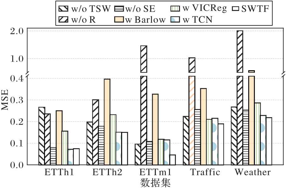
图2 SWTF各组件的消融实验结果
Fig. 2 Ablation study results of various components in SWTF
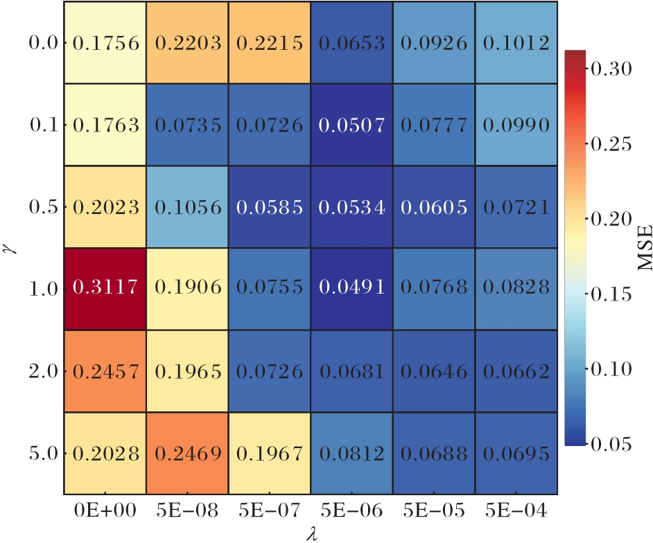
图3 TSW损失中权重对模型性能影响
Fig. 3 Impact of weights in TSW loss on model performance
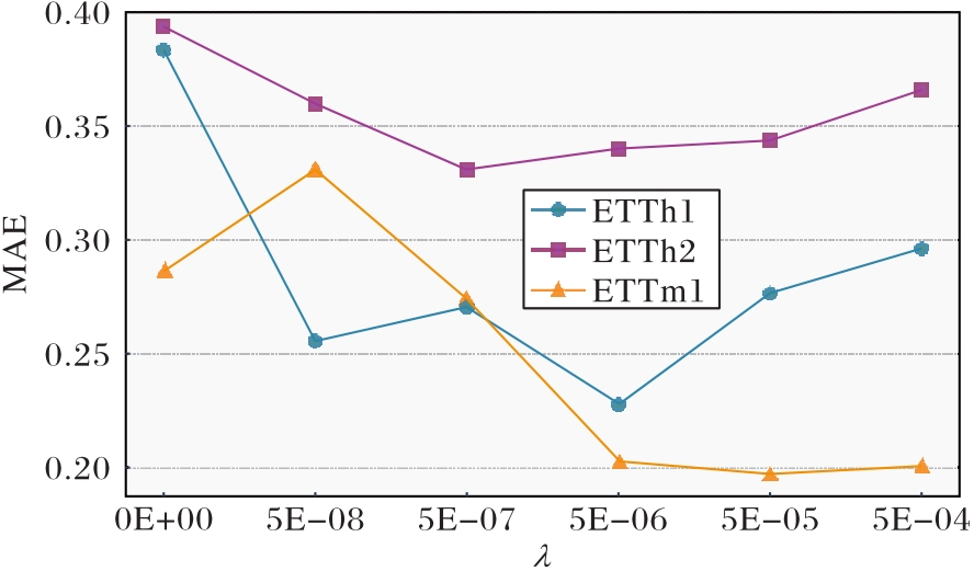
图4 TSW损失中权重λ在不同数据集上对性能的影响趋势
Fig. 4 Performance impact trends of weight λ in TSW loss on different datasets
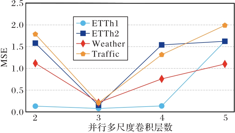
图5 并行多尺度卷积中卷积层数对模型性能的影响
Fig. 5 Impact of number of convolutional layers in parallel multi-scale convolution on model performance
| 模型 | GPU显存/GB | FLOPs/109 | 参数量/106 |
|---|---|---|---|
| SimTS | 2.7 | 349.86 | 104.76 |
| TimesURL | 7.9 | 1.90 | 0.60 |
| CoST | 2.8 | 11.57 | 27.49 |
| SWTF | 0.8 | 3.03 | 1.33 |
表3 计算成本对比
Tab. 3 Comparison of computational costs
| 模型 | GPU显存/GB | FLOPs/109 | 参数量/106 |
|---|---|---|---|
| SimTS | 2.7 | 349.86 | 104.76 |
| TimesURL | 7.9 | 1.90 | 0.60 |
| CoST | 2.8 | 11.57 | 27.49 |
| SWTF | 0.8 | 3.03 | 1.33 |
| 损失函数 | 表征质量 | 预测MSE | ||
|---|---|---|---|---|
| 平均家族内聚度 | 平均变体敏感度 | 平均家族间分离度 | ||
| TSW | 0.374 5 | 0.468 2 | 2.264 1 | 0.076 5 |
| Barlow | 0.003 0 | 0.003 5 | 0.008 2 | 0.324 1 |
| VICReg | 0.225 2 | 0.258 0 | 2.269 4 | 0.178 3 |
表4 不同损失函数下的表征质量与下游预测性能对比
Tab. 4 Comparison of representation quality and downstream prediction performance under different loss functions
| 损失函数 | 表征质量 | 预测MSE | ||
|---|---|---|---|---|
| 平均家族内聚度 | 平均变体敏感度 | 平均家族间分离度 | ||
| TSW | 0.374 5 | 0.468 2 | 2.264 1 | 0.076 5 |
| Barlow | 0.003 0 | 0.003 5 | 0.008 2 | 0.324 1 |
| VICReg | 0.225 2 | 0.258 0 | 2.269 4 | 0.178 3 |
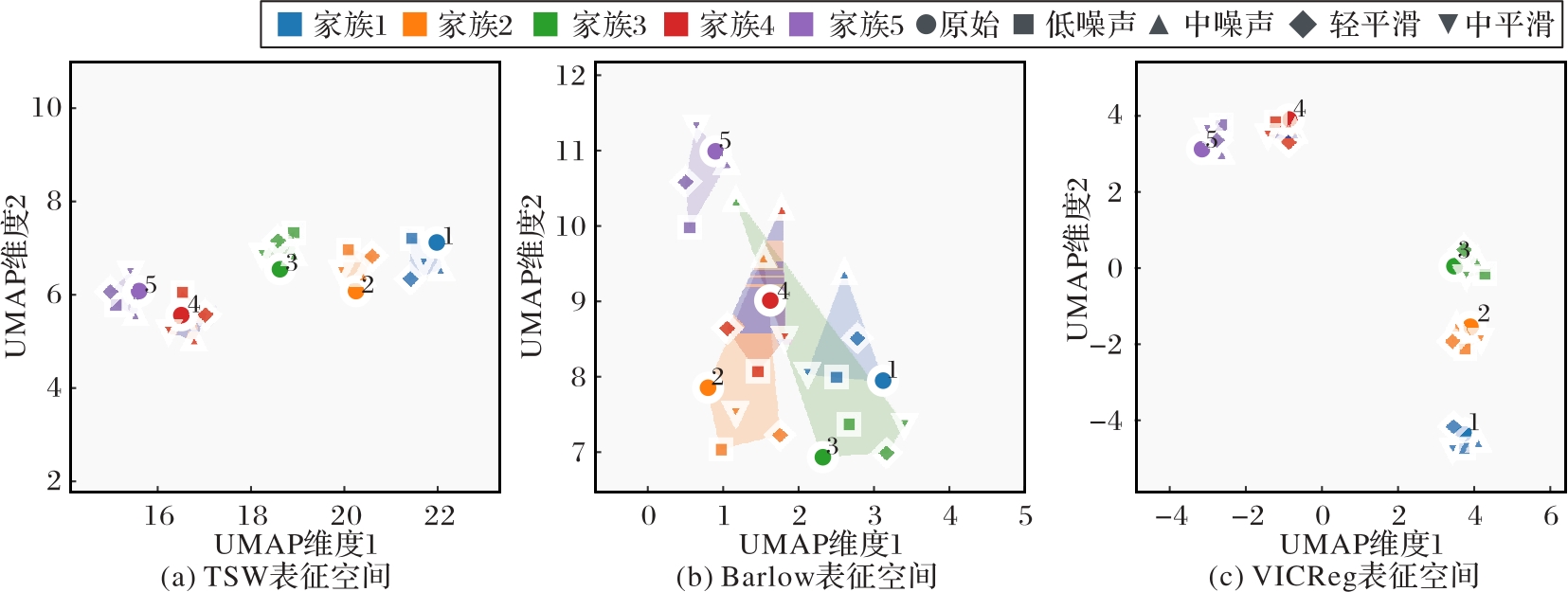
图6 3种损失函数下的表征空间UMAP可视化
Fig. 6 UMAP visualization of feature space under three loss functions
| 增强方法 | MSE | MAE |
|---|---|---|
| 高斯噪声 | 0.083 8 | 0.224 2 |
| 掩码 | 0.105 3 | 0.253 9 |
| 高斯噪声+掩码 | 0.107 1 | 0.256 9 |
| 椒盐噪声 | 0.124 5 | 0.277 4 |
| 椒盐噪声+掩码 | 0.157 2 | 0.322 0 |
表5 不同数据增强策略对性能的影响
Tab. 5 Impact of different data augmentation strategies on performance
| 增强方法 | MSE | MAE |
|---|---|---|
| 高斯噪声 | 0.083 8 | 0.224 2 |
| 掩码 | 0.105 3 | 0.253 9 |
| 高斯噪声+掩码 | 0.107 1 | 0.256 9 |
| 椒盐噪声 | 0.124 5 | 0.277 4 |
| 椒盐噪声+掩码 | 0.157 2 | 0.322 0 |
| 数据集 | 模型 | 高斯噪声(σ=0.1) | 掩码(r=0.05) | 椒盐噪声(p=0.1) | |||
|---|---|---|---|---|---|---|---|
| MAE | MSE | MAE | MSE | MAE | MSE | ||
| ETTh1 | CoST | 0.268 4 | 0.122 4 | 0.293 5 | 0.142 0 | 0.424 4 | 0.260 2 |
| TS2Vec | 0.269 0 | 0.124 2 | 0.311 7 | 0.168 4 | 0.493 2 | 0.463 6 | |
| SWTF | 0.225 3 | 0.084 3 | 0.241 4 | 0.095 5 | 0.222 1 | 0.081 8 | |
| ETTm1 | CoST | 0.182 3 | 0.062 2 | 0.213 5 | 0.081 8 | 0.334 4 | 0.185 8 |
| TS2Vec | 0.245 1 | 0.078 0 | 0.258 7 | 0.137 0 | 0.561 5 | 0.711 4 | |
| SWTF | 0.183 1 | 0.062 1 | 0.213 3 | 0.078 2 | 0.180 0 | 0.059 5 | |
| PEMS08 | CoST | 0.305 3 | 0.190 5 | 0.314 9 | 0.200 1 | 0.484 4 | 0.436 5 |
| TS2Vec | 0.277 4 | 0.148 0 | 0.290 0 | 0.172 0 | 0.567 4 | 0.653 2 | |
| SWTF | 0.229 8 | 0.114 8 | 0.233 1 | 0.116 7 | 0.276 5 | 0.145 9 | |
表6 扰动下各模型的下游预测任务性能对比
Tab. 6 Performance comparison of various models on downstream prediction tasks under perturbations
| 数据集 | 模型 | 高斯噪声(σ=0.1) | 掩码(r=0.05) | 椒盐噪声(p=0.1) | |||
|---|---|---|---|---|---|---|---|
| MAE | MSE | MAE | MSE | MAE | MSE | ||
| ETTh1 | CoST | 0.268 4 | 0.122 4 | 0.293 5 | 0.142 0 | 0.424 4 | 0.260 2 |
| TS2Vec | 0.269 0 | 0.124 2 | 0.311 7 | 0.168 4 | 0.493 2 | 0.463 6 | |
| SWTF | 0.225 3 | 0.084 3 | 0.241 4 | 0.095 5 | 0.222 1 | 0.081 8 | |
| ETTm1 | CoST | 0.182 3 | 0.062 2 | 0.213 5 | 0.081 8 | 0.334 4 | 0.185 8 |
| TS2Vec | 0.245 1 | 0.078 0 | 0.258 7 | 0.137 0 | 0.561 5 | 0.711 4 | |
| SWTF | 0.183 1 | 0.062 1 | 0.213 3 | 0.078 2 | 0.180 0 | 0.059 5 | |
| PEMS08 | CoST | 0.305 3 | 0.190 5 | 0.314 9 | 0.200 1 | 0.484 4 | 0.436 5 |
| TS2Vec | 0.277 4 | 0.148 0 | 0.290 0 | 0.172 0 | 0.567 4 | 0.653 2 | |
| SWTF | 0.229 8 | 0.114 8 | 0.233 1 | 0.116 7 | 0.276 5 | 0.145 9 | |
| 数据 | L | CoST | TS2Vec | SWTF | |||
|---|---|---|---|---|---|---|---|
| MAE | MSE | MAE | MSE | MAE | MSE | ||
| ETTh1 | 48 | 0.464 8 | 0.447 9 | 0.554 8 | 0.659 1 | 0.373 1 | 0.340 2 |
| 168 | 0.575 3 | 0.630 2 | 0.632 2 | 0.780 6 | 0.417 7 | 0.417 4 | |
| 336 | 0.659 3 | 0.794 8 | 0.691 9 | 0.888 6 | 0.446 5 | 0.464 9 | |
| 720 | 0.766 4 | 1.023 1 | 0.795 8 | 1.119 0 | 0.497 7 | 0.496 1 | |
| ETTh2 | 48 | 0.589 1 | 0.622 8 | 0.605 1 | 0.711 3 | 0.305 2 | 0.235 3 |
| 168 | 0.789 5 | 1.176 1 | 0.865 7 | 1.422 8 | 0.399 8 | 0.367 8 | |
| 336 | 0.887 0 | 1.477 0 | 0.998 6 | 1.854 3 | 0.453 4 | 0.442 8 | |
| 720 | 1.003 3 | 1.820 0 | 1.070 3 | 2.013 0 | 0.544 7 | 0.585 9 | |
| ETTm1 | 48 | 0.373 4 | 0.324 5 | 0.523 2 | 0.601 6 | 0.326 2 | 0.281 5 |
| 96 | 0.396 4 | 0.359 1 | 0.548 4 | 0.640 8 | 0.340 7 | 0.306 7 | |
| 288 | 0.459 4 | 0.449 9 | 0.605 6 | 0.726 8 | 0.378 3 | 0.371 4 | |
| 672 | 0.546 7 | 0.590 0 | 0.659 1 | 0.810 0 | 0.415 9 | 0.434 0 | |
表7 多变量预测结果
Tab. 7 Multivariate prediction results
| 数据 | L | CoST | TS2Vec | SWTF | |||
|---|---|---|---|---|---|---|---|
| MAE | MSE | MAE | MSE | MAE | MSE | ||
| ETTh1 | 48 | 0.464 8 | 0.447 9 | 0.554 8 | 0.659 1 | 0.373 1 | 0.340 2 |
| 168 | 0.575 3 | 0.630 2 | 0.632 2 | 0.780 6 | 0.417 7 | 0.417 4 | |
| 336 | 0.659 3 | 0.794 8 | 0.691 9 | 0.888 6 | 0.446 5 | 0.464 9 | |
| 720 | 0.766 4 | 1.023 1 | 0.795 8 | 1.119 0 | 0.497 7 | 0.496 1 | |
| ETTh2 | 48 | 0.589 1 | 0.622 8 | 0.605 1 | 0.711 3 | 0.305 2 | 0.235 3 |
| 168 | 0.789 5 | 1.176 1 | 0.865 7 | 1.422 8 | 0.399 8 | 0.367 8 | |
| 336 | 0.887 0 | 1.477 0 | 0.998 6 | 1.854 3 | 0.453 4 | 0.442 8 | |
| 720 | 1.003 3 | 1.820 0 | 1.070 3 | 2.013 0 | 0.544 7 | 0.585 9 | |
| ETTm1 | 48 | 0.373 4 | 0.324 5 | 0.523 2 | 0.601 6 | 0.326 2 | 0.281 5 |
| 96 | 0.396 4 | 0.359 1 | 0.548 4 | 0.640 8 | 0.340 7 | 0.306 7 | |
| 288 | 0.459 4 | 0.449 9 | 0.605 6 | 0.726 8 | 0.378 3 | 0.371 4 | |
| 672 | 0.546 7 | 0.590 0 | 0.659 1 | 0.810 0 | 0.415 9 | 0.434 0 | |
| [1] | Oreshkin B N, Carpov D, Chapados N, et al. N-BEATS: neural basis expansion analysis for interpretable time series forecasting[PP/OL]. V4. arXiv (2020-02-20) [2025-10-11].. |
| [2] | Salinas D, Flunkert V, Gasthaus J, et al. DeepAR: probabilistic forecasting with autoregressive recurrent networks[J]. International Journal of Forecasting, 2020, 36(3): 1181-1191. |
| [3] | 李嘉源,王晓东,何启学. CNN增强型Informer模型在工业时间序列预测中的应用及性能优化[J]. 计算机应用, 2024, 44(S2): 79-83. |
| Li Jiayuan, Wang Xiaodong, He Qixue. Application and performance optimization of CNN enhanced Informer model in industrial time series prediction[J]. Journal of Computer Applications, 2024, 44(S2): 79-83. | |
| [4] | Liu P, Wu B, Hu Y, et al. TimeBridge: non-stationarity matters for long-term time series forecasting[J]. Proceedings of International Conference on Machine Learning, 2025, 267: 39815-39840. |
| [5] | Zhang K, Wen Q, Zhang C, et al. Self-supervised learning for time series analysis: taxonomy, progress, and prospects[J]. IEEE Transactions on Pattern Analysis and Machine Intelligence, 2024, 46(10): 6775-6794. |
| [6] | He K, Fan H, Wu Y, et al. Momentum contrast for unsupervised visual representation learning[C]// CVPR 2020. Piscataway: IEEE, 2020: 9726-9735. |
| [7] | Chen X, He K. Exploring simple Siamese representation learning[C]// CVPR 2021. Piscataway: IEEE, 2021: 15745-15753. |
| [8] | Tian Y, Sun C, Poole B, et al. What makes for good views for contrastive learning?[C]// NeurIPS 2020. Red Hook: Curran Associates Inc., 2020: 6827-6839. |
| [9] | Liu J, Chen S. TimesURL: self-supervised contrastive learning for universal time series representation learning[J]. Proceedings of the AAAI Conference on Artificial Intelligence, 2024, 38(12): 13918-13926. |
| [10] | Luo D, Cheng W, Wang Y, et al. Time series contrastive learning with information-aware augmentations[J]. Proceedings of the AAAI Conference on Artificial Intelligence, 2023, 37(4): 4534-4542. |
| [11] | Bai S, Kolter J Z, Koltun V. An empirical evaluation of generic convolutional and recurrent networks for sequence modeling[PP/OL]. V2. arXiv (2018-04-19) [2025-10-11].. |
| [12] | Zhou T, Ma Z, Wen Q, et al. FEDformer: frequency enhanced decomposed transformer for long-term series forecasting[J]. Proceedings of Machine Learning Research, 2022, 162: 27268-27286. |
| [13] | Zhou H, Zhang S, Peng J, et al. Informer: beyond efficient Transformer for long sequence time-series forecasting[J]. Proceedings of the AAAI Conference on Artificial Intelligence, 2021, 35(12): 11106-11115. |
| [14] | Wu H, Xu J, Wang J, et al. Autoformer: decomposition Transformers with auto-correlation for long-term series forecasting[C]// NeurIPS 2021. Red Hook: Curran Associates Inc., 2021: 22419-22430. |
| [15] | van den Oord A, Li Y, Vinyals O. Representation learning with contrastive predictive coding[PP/OL]. V2. arXiv (2019-01-22) [2025-10-11].. |
| [16] | Eldele E, Ragab M, Chen Z, et al. Time-series representation learning via temporal and contextual contrasting[C]// IJCAI 2021. California: ijcai.org, 2021: 2352-2359. |
| [17] | Tonekaboni S, Eytan D, Goldenberg A. Unsupervised representation learning for time series with temporal neighborhood coding[PP/OL]. V1. arXiv (2021-07-01) [2025-10-11].. |
| [18] | Yue Z, Wang Y, Duan J, et al. TS2Vec: towards universal representation of time series[J]. Proceedings of the AAAI Conference on Artificial Intelligence, 2022, 36(8): 8980-8987. |
| [19] | Woo G, Liu C, Sahoo D, et al. CoST: contrastive learning of disentangled seasonal-trend representations for time series forecasting[PP/OL]. V3. arXiv (2022-05-05) [2025-10-11].. |
| [20] | Zhang X, Zhao Z, Tsiligkaridis T, et al. Self-supervised contrastive pre-training for time series via time-frequency consistency[C]// NeurIPS 2022. Red Hook: Curran Associates Inc., 2022: 3988-4003. |
| [21] | Yang X, Zhang Z, Cui R. TimeCLR: a self-supervised contrastive learning framework for univariate time series representation[J]. Knowledge-Based Systems, 2022, 245: No.108606. |
| [22] | Liu K J, Suganuma M, Okatani T. Bridging the gap from asymmetry tricks to decorrelation principles in non-contrastive self-supervised learning[C]// NeurIPS 2022. Red Hook: Curran Associates Inc., 2022: 19824-19835. |
| [23] | Zhang Y, Zhu H, Song Z, et al. Geometric view of soft decorrelation in self-supervised learning[C]// KDD 2024. New York: ACM, 2024: 4338-4349. |
| [24] | Grill J B, Strub F, Altché F, et al. Bootstrap your own latent: a new approach to self-supervised learning[C]// NeurIPS 2020. Red Hook: Curran Associates Inc., 2020: 21271-21284. |
| [25] | Zbontar J, Jing L, Misra I, et al. Barlow Twins: self-supervised learning via redundancy reduction[J]. Proceedings of Machine Learning Research, 2021, 139: 12310-12320. |
| [26] | Bardes A, Ponce J, LeCun Y. VICReg: variance-invariance-covariance regularization for self-supervised learning[PP/OL]. V3. arXiv (2022-01-28) [2025-10-11].. |
| [27] | Ermolov A, Siarohin A, Sangineto E, et al. Whitening for self-supervised representation learning[J]. Proceedings of Machine Learning Research, 2021, 139: 3015-3024. |
| [28] | Hua T, Wang W, Xue Z, et al. On feature decorrelation in self-supervised learning[C]// ICCV 2021. Piscataway: IEEE, 2021: 9578-9588. |
| [29] | Fu E, Hu Y. Frequency-masked embedding inference: a non-contrastive approach for time series representation learning[J]. Proceedings of the AAAI Conference on Artificial Intelligence, 2025, 39(16): 16639-16647. |
| [30] | Zhang W, Yang L, Geng S, et al. Self-supervised time series representation learning via cross reconstruction Transformer[J]. IEEE Transactions on Neural Networks and Learning Systems, 2024, 35(11): 16129-16138. |
| [31] | Lee S, Park T, Lee K. Soft contrastive learning for time series[PP/OL]. V3. arXiv (2024-03-22) [2025-10-11].. |
| [32] | Dai T, Wu B, Liu P, et al. Periodicity decoupling framework for long-term series forecasting[EB/OL]. (2024-03-06) [2025-10-11].. |
| [33] | Fraikin A, Bennetot A, Allassonnière S. T-Rep: representation learning for time series using time-embeddings[PP/OL]. V3. arXiv (2024-05-09) [2025-10-11].. |
| [34] | Kim T, Kim J, Tae Y, et al. Reversible instance normalization for accurate time-series forecasting against distribution shift[EB/OL]. (2023-02-14) [2025-10-11].. |
| [35] | McInnes L, Healy J, Melville J. UMAP: uniform manifold approximation and projection for dimension reduction[PP/OL]. V2. arXiv (2020-09-18) [2025-10-11]. . |
| [1] | 王岩, 陈曦, 赵中恺, 周欢, 吴涛, 艾梦格, 肖雪松. 相似度感知的民族文化知识图谱链路预测模型[J]. 《计算机应用》唯一官方网站, 2026, 46(8): 2447-2456. |
| [2] | 李光辉, 屈立成. 基于改进Lite-Mono架构的动态空洞卷积和分层注意力模型[J]. 《计算机应用》唯一官方网站, 2026, 46(8): 2567-2576. |
| [3] | 吕慧慧, 仲兆满, 张渝, 樊继冬. 融合互信息最大化与对比学习的句法增强型方面级情感分析[J]. 《计算机应用》唯一官方网站, 2026, 46(8): 2440-2446. |
| [4] | 王昱麒, 张仰森, 王璞. 融合知识增强和对比学习的高中英语阅读理解模型[J]. 《计算机应用》唯一官方网站, 2026, 46(7): 2096-2103. |
| [5] | 樊海玮, 丁文帅, 邢宏政. 基于多异构拓扑图协同与层次对比学习的知识感知推荐性能增强方法[J]. 《计算机应用》唯一官方网站, 2026, 46(7): 2085-2095. |
| [6] | 陈宇, 戚帅康, 许莉薇, 朱浩天. 融合多尺度小波增强与自监督学习的社交机器人检测框架[J]. 《计算机应用》唯一官方网站, 2026, 46(6): 1756-1766. |
| [7] | 李冰清, 黄彬浩, 唐语蓓, 张柏礼. 面向数据稀疏性与冷启动问题的服务质量预测模型[J]. 《计算机应用》唯一官方网站, 2026, 46(6): 1829-1835. |
| [8] | 戚航, 董婷婷, 乃永强, 莫先. 基于图扩散生成与自适应采样的对比协同过滤方法[J]. 《计算机应用》唯一官方网站, 2026, 46(6): 1818-1828. |
| [9] | 王静红, 陈潇, 马迎梅, 李笔, 米据生, 王威. 基于自适应学习的多层次邻域对比属性图聚类[J]. 《计算机应用》唯一官方网站, 2026, 46(6): 1836-1843. |
| [10] | 喻小芹, 单武扬, 邱骏颖, 林宇, 杨容浩, 田茂. 亮度对比度扰动下的图像篡改定位检测网络[J]. 《计算机应用》唯一官方网站, 2026, 46(6): 1893-1903. |
| [11] | 袁浩然, 刘欢, 焦鹏飞, 赵治栋, 张显飞, 柳遵梁. 掩码自编码器增强的动态异质图表示学习模型[J]. 《计算机应用》唯一官方网站, 2026, 46(6): 1728-1737. |
| [12] | 富坤, 魏昊宇, 刘伟静, 党兴, 刘泽政, 李建伟. 拓扑语义双域协同的图神经网络框架[J]. 《计算机应用》唯一官方网站, 2026, 46(5): 1378-1387. |
| [13] | 张棣锐, 林佳瑜, 梁祖红. 基于不确定性感知非似然学习的监督对比生成式情感分析方法[J]. 《计算机应用》唯一官方网站, 2026, 46(5): 1416-1423. |
| [14] | 赵海华, 胡怡君, 唐瑞, 莫先. 基于语义融合和对比增强的多模态推荐方法[J]. 《计算机应用》唯一官方网站, 2026, 46(4): 1058-1068. |
| [15] | 刘晓霞, 况立群, 王松, 焦世超, 韩慧妍, 熊风光. 多尺度时空解耦的骨架行为识别对比学习[J]. 《计算机应用》唯一官方网站, 2026, 46(3): 767-774. |
| 阅读次数 | ||||||
|
全文 |
|
|||||
|
摘要 |
|
|||||
