


《计算机应用》唯一官方网站 ›› 2025, Vol. 45 ›› Issue (10): 3381-3389.DOI: 10.11772/j.issn.1001-9081.2024101501
• 前沿与综合应用 • 上一篇
高照耀1,2, 张展2( ), 胡亮亮3, 许光宇1, 周胜4, 胡雨欣1,2, 林子捷5, 周超2,5
收稿日期:2024-10-24
修回日期:2025-01-10
接受日期:2025-01-16
发布日期:2025-02-07
出版日期:2025-10-10
通讯作者:
张展
作者简介:高照耀(1999—),男,安徽滁州人,硕士研究生,主要研究方向:信号处理、核磁共振图像重建基金资助:
Zhaoyao GAO1,2, Zhan ZHANG2(), Liangliang HU3, Guangyu XU1, Sheng ZHOU4, Yuxin HU1,2, Zijie LIN5, Chao ZHOU2,5
Received:2024-10-24
Revised:2025-01-10
Accepted:2025-01-16
Online:2025-02-07
Published:2025-10-10
Contact:
Zhan ZHANG
About author:GAO Zhaoyao, born in 1999, M. S. candidate. His research interests include signal processing, magnetic resonance imaging reconstruction.Supported by:摘要:
并行成像技术可以帮助解决超高场强磁共振成像(MRI)中的射频能量沉积、图像均匀性的问题,缩短扫描时间,减少运动伪影,并提升数据采集速度。为了提高对MRI复值数据的特征提取能力,减少并行成像欠采样所引起的卷褶伪影,提出基于K空间插值的残差复卷积鲁棒人工神经网络(RCRAKI)。所提算法将原始欠采样MRI扫描数据作为输入,利用残差结构结合线性与非线性重建方法的优势,在残差连接部分利用卷积创建线性重建基线,主路径利用多层复卷积补偿基线缺陷,最终重建出伪影更少的磁共振(MR)图像。在合肥综合性国家科学中心能源研究院自主研发的7T超高场磁共振设备采集的数据上进行实验,并将RCRAKI与基于K空间插值的残差鲁棒人工神经网络(rRAKI)在自动校准信号(ACS)数为40、加速比为8的采样率下进行小鼠不同解剖切面成像质量对比。实验结果表明:在矢状位下,所提算法的标准化均方根误差(NRMSE)指标下降了59.74%,结构相似度(SSIM)指标提升了0.45%,峰值信噪比(PSNR)指标提升了13.04%;在横断位下,所提算法的NRMSE指标降低了7.97%,SSIM指标略有改善(提高了0.005%),PSNR指标提升了1.09%;在冠状位下,所提算法的NRMSE指标下降了35.03%,PSNR指标提升了5.60%,SSIM指标提升了0.98%。可见,RCRAKI在不同解剖切面的MRI数据上均表现出良好的性能,在高加速比采样率下能够减小噪声放大的影响,并重建出细节更清晰的MR图像。
中图分类号:
高照耀, 张展, 胡亮亮, 许光宇, 周胜, 胡雨欣, 林子捷, 周超. 基于残差复卷积网络的7T超高场磁共振并行成像算法[J]. 计算机应用, 2025, 45(10): 3381-3389.
Zhaoyao GAO, Zhan ZHANG, Liangliang HU, Guangyu XU, Sheng ZHOU, Yuxin HU, Zijie LIN, Chao ZHOU. 7T ultra-high field magnetic resonance parallel imaging algorithm based on residual complex convolution network[J]. Journal of Computer Applications, 2025, 45(10): 3381-3389.
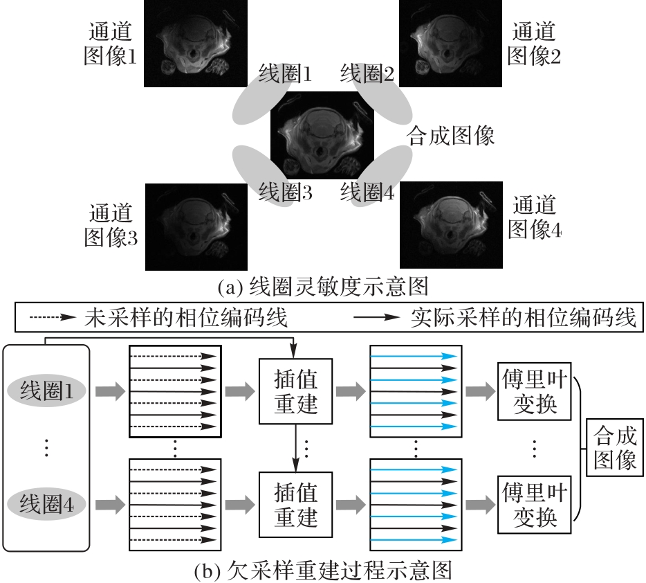
图1 磁共振并行成像原理
Fig. 1 Principle of magnetic resonance parallel imaging
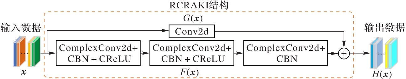
图2 RCRAKI的整体架构
Fig. 2 Overall architecture of RCRAKI
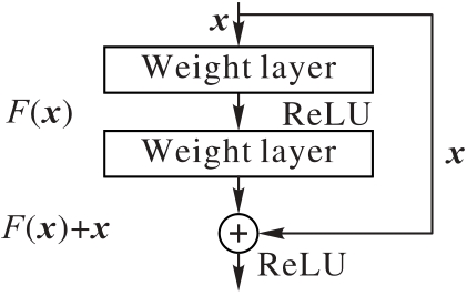
图3 残差结构
Fig. 3 Residual structure
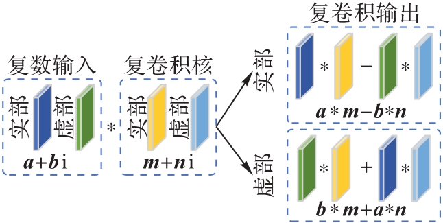
图4 复卷积示例
Fig. 4 Example of complex convolution
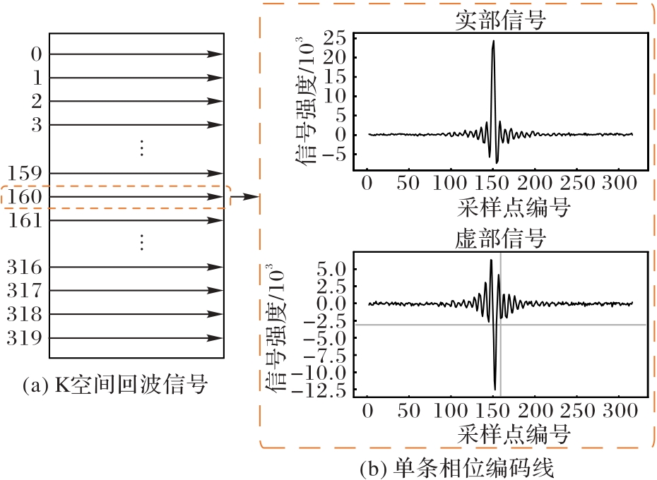
图5 相位编码线示例
Fig. 5 Example of phase encoding line
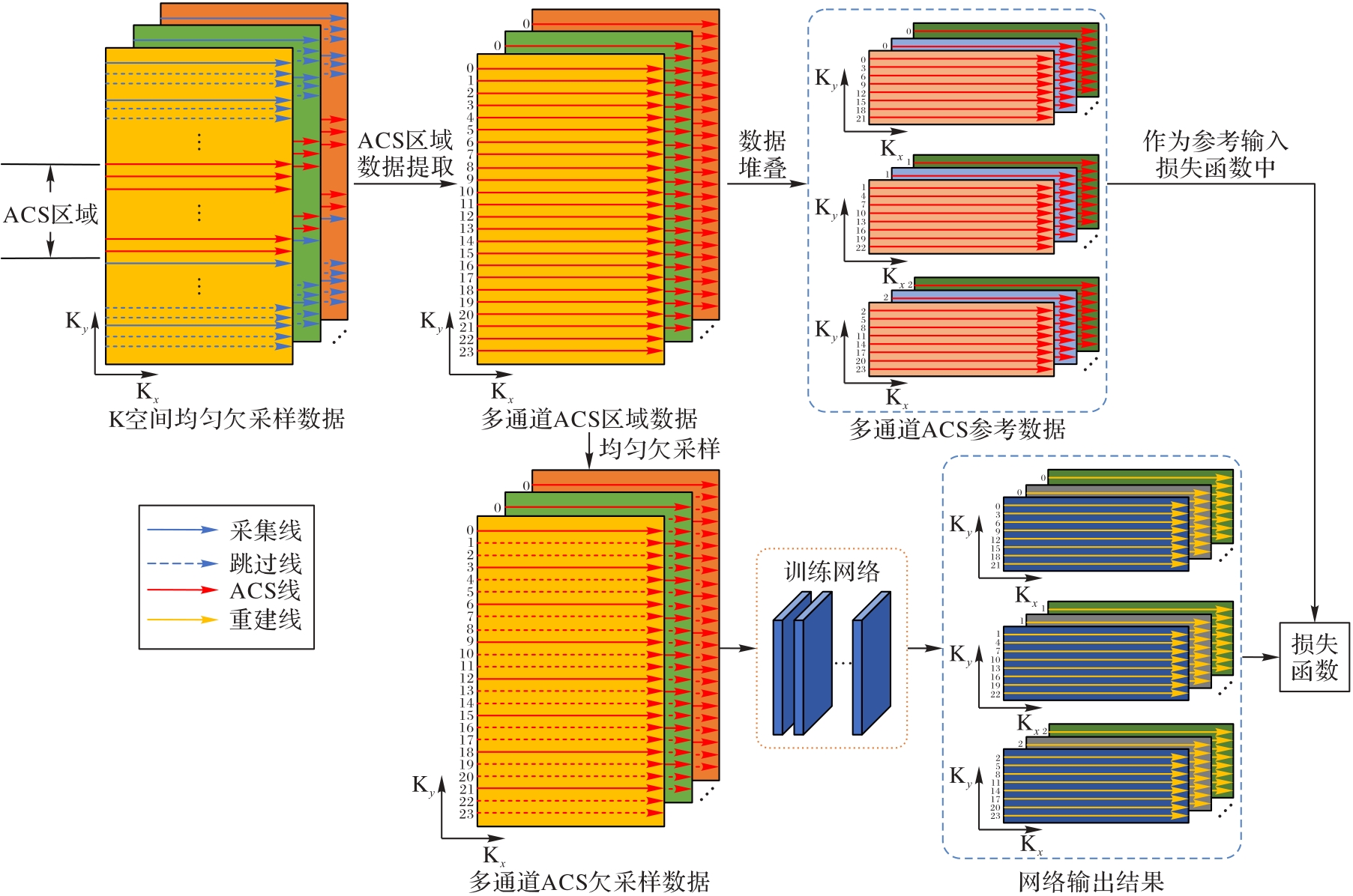
图6 RCRAKI的训练流程
Fig. 6 Training process of RCRAKI
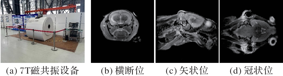
图7 7T磁共振的数据样本
Fig. 7 Data samples of 7T magnetic resonance
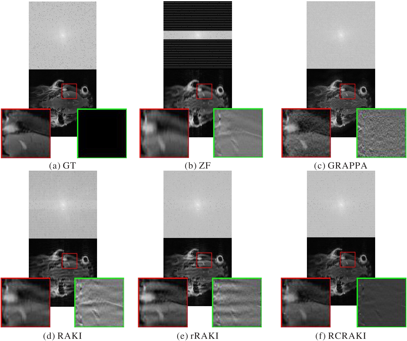
图8 小鼠冠状位重建结果的对比
Fig. 8 Comparison of coronal plane reconstruction results of mouse
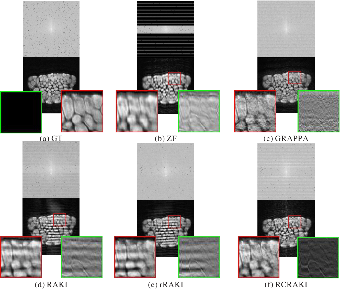
图9 橘瓣冠状位重建结果的对比
Fig. 9 Comparison of coronal plane reconstruction results of orange segment
| 采样模式 | 算法 | NRMSE | SSIM | PSNR/dB | |
|---|---|---|---|---|---|
| NACS | rate | ||||
| 30 | 2 | ZF | 0.142 458 01 | 0.915 087 82 | 23.902 764 04 |
| GRAPPA | 0.003 541 90 | 0.972 988 01 | 39.990 581 44 | ||
| RAKI | 0.007 244 31 | 0.973 258 07 | 36.839 659 80 | ||
| rRAKI | 0.003 688 19 | 0.974 834 25 | 39.818 398 06 | ||
| RCRAKI | 0.003 418 73 | 0.975 292 60 | 40.035 774 10 | ||
| 3 | ZF | 0.202 789 48 | 0.886 558 14 | 22.520 205 89 | |
| GRAPPA | 0.007 667 29 | 0.954 258 17 | 36.636 524 31 | ||
| RAKI | 0.034 356 36 | 0.953 532 86 | 30.230 589 10 | ||
| rRAKI | 0.009 670 57 | 0.957 742 94 | 35.970 478 28 | ||
| RCRAKI | 0.006 940 29 | 0.957 969 19 | 37.176 881 87 | ||
| 40 | 2 | ZF | 0.127 766 00 | 0.926 240 51 | 24.267 329 98 |
| GRAPPA | 0.003 187 30 | 0.976 947 79 | 40.448 718 44 | ||
| RAKI | 0.003 727 72 | 0.974 463 85 | 40.165 202 34 | ||
| rRAKI | 0.003 251 53 | 0.972 707 06 | 40.365 474 12 | ||
| RCRAKI | 0.003 123 91 | 0.975 651 90 | 40.492 646 53 | ||
| 4 | ZF | 0.210 604 28 | 0.888 745 30 | 22.204 960 71 | |
| GRAPPA | 0.019 037 45 | 0.906 617 11 | 32.686 857 65 | ||
| RAKI | 0.052 912 92 | 0.934 690 09 | 28.828 713 09 | ||
| rRAKI | 0.024 772 03 | 0.937 842 32 | 31.415 594 25 | ||
| RCRAKI | 0.018 092 50 | 0.944 431 33 | 32.731 004 45 | ||
| 8 | ZF | 0.200 982 87 | 0.880 228 27 | 22.408 042 13 | |
| GRAPPA | 0.085 235 68 | 0.779 268 26 | 26.176 731 60 | ||
| RAKI | 0.157 800 38 | 0.870 278 07 | 23.458 552 16 | ||
| rRAKI | 0.081 201 84 | 0.888 080 79 | 26.851 648 46 | ||
| RCRAKI | 0.032 691 56 | 0.892 073 63 | 30.352 650 32 | ||
表1 不同采样模式与算法下的小鼠矢状位重建结果的定量比较
Tab. 1 Quantitative comparison of sagittal plane reconstruction results of mouse using different algorithms under various sampling modes
| 采样模式 | 算法 | NRMSE | SSIM | PSNR/dB | |
|---|---|---|---|---|---|
| NACS | rate | ||||
| 30 | 2 | ZF | 0.142 458 01 | 0.915 087 82 | 23.902 764 04 |
| GRAPPA | 0.003 541 90 | 0.972 988 01 | 39.990 581 44 | ||
| RAKI | 0.007 244 31 | 0.973 258 07 | 36.839 659 80 | ||
| rRAKI | 0.003 688 19 | 0.974 834 25 | 39.818 398 06 | ||
| RCRAKI | 0.003 418 73 | 0.975 292 60 | 40.035 774 10 | ||
| 3 | ZF | 0.202 789 48 | 0.886 558 14 | 22.520 205 89 | |
| GRAPPA | 0.007 667 29 | 0.954 258 17 | 36.636 524 31 | ||
| RAKI | 0.034 356 36 | 0.953 532 86 | 30.230 589 10 | ||
| rRAKI | 0.009 670 57 | 0.957 742 94 | 35.970 478 28 | ||
| RCRAKI | 0.006 940 29 | 0.957 969 19 | 37.176 881 87 | ||
| 40 | 2 | ZF | 0.127 766 00 | 0.926 240 51 | 24.267 329 98 |
| GRAPPA | 0.003 187 30 | 0.976 947 79 | 40.448 718 44 | ||
| RAKI | 0.003 727 72 | 0.974 463 85 | 40.165 202 34 | ||
| rRAKI | 0.003 251 53 | 0.972 707 06 | 40.365 474 12 | ||
| RCRAKI | 0.003 123 91 | 0.975 651 90 | 40.492 646 53 | ||
| 4 | ZF | 0.210 604 28 | 0.888 745 30 | 22.204 960 71 | |
| GRAPPA | 0.019 037 45 | 0.906 617 11 | 32.686 857 65 | ||
| RAKI | 0.052 912 92 | 0.934 690 09 | 28.828 713 09 | ||
| rRAKI | 0.024 772 03 | 0.937 842 32 | 31.415 594 25 | ||
| RCRAKI | 0.018 092 50 | 0.944 431 33 | 32.731 004 45 | ||
| 8 | ZF | 0.200 982 87 | 0.880 228 27 | 22.408 042 13 | |
| GRAPPA | 0.085 235 68 | 0.779 268 26 | 26.176 731 60 | ||
| RAKI | 0.157 800 38 | 0.870 278 07 | 23.458 552 16 | ||
| rRAKI | 0.081 201 84 | 0.888 080 79 | 26.851 648 46 | ||
| RCRAKI | 0.032 691 56 | 0.892 073 63 | 30.352 650 32 | ||
| 采样模式 | 算法 | NRMSE | SSIM | PSNR/dB | |
|---|---|---|---|---|---|
| NACS | rate | ||||
| 30 | 2 | ZF | 0.211 770 56 | 0.912 599 84 | 24.521 678 76 |
| GRAPPA | 0.002 643 45 | 0.979 180 56 | 43.558 617 44 | ||
| RAKI | 0.004 877 09 | 0.975 954 82 | 40.898 720 70 | ||
| rRAKI | 0.002 120 70 | 0.986 610 08 | 44.515 535 79 | ||
| RCRAKI | 0.002 115 99 | 0.986 735 50 | 44.525 187 70 | ||
| 3 | ZF | 0.302 426 83 | 0.902 198 04 | 22.753 947 17 | |
| GRAPPA | 0.005 269 48 | 0.956 157 82 | 40.562 653 78 | ||
| RAKI | 0.016 427 03 | 0.963 051 33 | 35.404 559 67 | ||
| rRAKI | 0.004 555 08 | 0.969 976 73 | 40.972 257 38 | ||
| RCRAKI | 0.004 863 32 | 0.974 765 66 | 40.690 430 18 | ||
| 40 | 2 | ZF | 0.145 095 88 | 0.938 843 77 | 26.163 783 79 |
| GRAPPA | 0.002 494 39 | 0.978 611 48 | 43.810 677 93 | ||
| RAKI | 0.003 309 85 | 0.973 819 37 | 42.582 248 75 | ||
| rRAKI | 0.002 100 74 | 0.985 028 08 | 44.556 403 15 | ||
| RCRAKI | 0.001 954 27 | 0.988 486 69 | 44.870 490 21 | ||
| 4 | ZF | 0.410 778 12 | 0.903 930 86 | 21.644 261 61 | |
| GRAPPA | 0.011 571 58 | 0.928 763 84 | 37.146 405 88 | ||
| RAKI | 0.012 008 34 | 0.962 025 96 | 36.985 504 06 | ||
| rRAKI | 0.008 300 74 | 0.962 333 01 | 38.589 163 75 | ||
| RCRAKI | 0.009 064 88 | 0.964 618 39 | 38.206 709 43 | ||
| 8 | ZF | 0.433 850 05 | 0.901 630 24 | 21.406 938 09 | |
| GRAPPA | 0.061 405 57 | 0.860 340 73 | 29.898 256 81 | ||
| RAKI | 0.055 075 52 | 0.932 176 01 | 30.370 748 11 | ||
| rRAKI | 0.028 887 94 | 0.946 611 09 | 33.173 168 66 | ||
| RCRAKI | 0.026 586 84 | 0.946 658 07 | 33.533 666 67 | ||
表2 不同采样模式与算法下的小鼠横断位重建结果的定量比较
Tab. 2 Quantitative comparison of axial plane reconstruction results of mouse using different algorithms under various sampling modes
| 采样模式 | 算法 | NRMSE | SSIM | PSNR/dB | |
|---|---|---|---|---|---|
| NACS | rate | ||||
| 30 | 2 | ZF | 0.211 770 56 | 0.912 599 84 | 24.521 678 76 |
| GRAPPA | 0.002 643 45 | 0.979 180 56 | 43.558 617 44 | ||
| RAKI | 0.004 877 09 | 0.975 954 82 | 40.898 720 70 | ||
| rRAKI | 0.002 120 70 | 0.986 610 08 | 44.515 535 79 | ||
| RCRAKI | 0.002 115 99 | 0.986 735 50 | 44.525 187 70 | ||
| 3 | ZF | 0.302 426 83 | 0.902 198 04 | 22.753 947 17 | |
| GRAPPA | 0.005 269 48 | 0.956 157 82 | 40.562 653 78 | ||
| RAKI | 0.016 427 03 | 0.963 051 33 | 35.404 559 67 | ||
| rRAKI | 0.004 555 08 | 0.969 976 73 | 40.972 257 38 | ||
| RCRAKI | 0.004 863 32 | 0.974 765 66 | 40.690 430 18 | ||
| 40 | 2 | ZF | 0.145 095 88 | 0.938 843 77 | 26.163 783 79 |
| GRAPPA | 0.002 494 39 | 0.978 611 48 | 43.810 677 93 | ||
| RAKI | 0.003 309 85 | 0.973 819 37 | 42.582 248 75 | ||
| rRAKI | 0.002 100 74 | 0.985 028 08 | 44.556 403 15 | ||
| RCRAKI | 0.001 954 27 | 0.988 486 69 | 44.870 490 21 | ||
| 4 | ZF | 0.410 778 12 | 0.903 930 86 | 21.644 261 61 | |
| GRAPPA | 0.011 571 58 | 0.928 763 84 | 37.146 405 88 | ||
| RAKI | 0.012 008 34 | 0.962 025 96 | 36.985 504 06 | ||
| rRAKI | 0.008 300 74 | 0.962 333 01 | 38.589 163 75 | ||
| RCRAKI | 0.009 064 88 | 0.964 618 39 | 38.206 709 43 | ||
| 8 | ZF | 0.433 850 05 | 0.901 630 24 | 21.406 938 09 | |
| GRAPPA | 0.061 405 57 | 0.860 340 73 | 29.898 256 81 | ||
| RAKI | 0.055 075 52 | 0.932 176 01 | 30.370 748 11 | ||
| rRAKI | 0.028 887 94 | 0.946 611 09 | 33.173 168 66 | ||
| RCRAKI | 0.026 586 84 | 0.946 658 07 | 33.533 666 67 | ||
| 采样模式 | 算法 | NRMSE | SSIM | PSNR/dB | |
|---|---|---|---|---|---|
| NACS | rate | ||||
| 30 | 2 | ZF | 0.055 123 71 | 0.959 548 79 | 33.172 203 32 |
| GRAPPA | 0.002 713 90 | 0.992 051 37 | 46.270 613 44 | ||
| RAKI | 0.003 545 20 | 0.991 787 10 | 45.089 176 06 | ||
| rRAKI | 0.002 631 07 | 0.993 117 37 | 46.384 379 77 | ||
| RCRAKI | 0.002 594 87 | 0.993 451 56 | 46.444 500 00 | ||
| 3 | ZF | 0.112 634 96 | 0.929 946 24 | 30.020 655 43 | |
| GRAPPA | 0.007 139 27 | 0.981 853 30 | 42.070 025 26 | ||
| RAKI | 0.010 104 12 | 0.980 954 10 | 40.492 387 14 | ||
| rRAKI | 0.005 730 24 | 0.985 881 26 | 42.955 433 68 | ||
| RCRAKI | 0.005 675 46 | 0.987 121 30 | 42.997 396 27 | ||
| 40 | 2 | ZF | 0.033 361 68 | 0.972 235 18 | 35.353 109 07 |
| GRAPPA | 0.002 573 55 | 0.992 027 74 | 46.501 233 27 | ||
| RAKI | 0.002 873 33 | 0.991 949 45 | 46.001 754 51 | ||
| rRAKI | 0.002 377 84 | 0.992 461 47 | 46.833 736 85 | ||
| RCRAKI | 0.002 371 69 | 0.993 160 54 | 46.835 004 86 | ||
| 4 | ZF | 0.077 271 58 | 0.947 333 11 | 31.705 390 53 | |
| GRAPPA | 0.018 849 08 | 0.957 162 85 | 37.853 659 80 | ||
| RAKI | 0.013 300 72 | 0.974 484 10 | 39.346 810 24 | ||
| rRAKI | 0.008 718 41 | 0.980 464 71 | 41.185 102 87 | ||
| RCRAKI | 0.009 801 50 | 0.980 654 14 | 40.672 661 27 | ||
| 8 | ZF | 0.121 397 84 | 0.932 714 97 | 29.743 478 68 | |
| GRAPPA | 0.084 294 66 | 0.880 373 03 | 31.348 562 93 | ||
| RAKI | 0.053 645 78 | 0.935 678 45 | 33.288 645 10 | ||
| rRAKI | 0.045 854 56 | 0.947 206 90 | 33.985 345 78 | ||
| RCRAKI | 0.029 791 42 | 0.956 521 47 | 35.887 412 78 | ||
表3 不同采样模式与算法下的小鼠冠状位重建结果的定量比较
Tab. 3 Quantitative comparison of coronal plane reconstruction results using mouse using different algorithms under various sampling modes
| 采样模式 | 算法 | NRMSE | SSIM | PSNR/dB | |
|---|---|---|---|---|---|
| NACS | rate | ||||
| 30 | 2 | ZF | 0.055 123 71 | 0.959 548 79 | 33.172 203 32 |
| GRAPPA | 0.002 713 90 | 0.992 051 37 | 46.270 613 44 | ||
| RAKI | 0.003 545 20 | 0.991 787 10 | 45.089 176 06 | ||
| rRAKI | 0.002 631 07 | 0.993 117 37 | 46.384 379 77 | ||
| RCRAKI | 0.002 594 87 | 0.993 451 56 | 46.444 500 00 | ||
| 3 | ZF | 0.112 634 96 | 0.929 946 24 | 30.020 655 43 | |
| GRAPPA | 0.007 139 27 | 0.981 853 30 | 42.070 025 26 | ||
| RAKI | 0.010 104 12 | 0.980 954 10 | 40.492 387 14 | ||
| rRAKI | 0.005 730 24 | 0.985 881 26 | 42.955 433 68 | ||
| RCRAKI | 0.005 675 46 | 0.987 121 30 | 42.997 396 27 | ||
| 40 | 2 | ZF | 0.033 361 68 | 0.972 235 18 | 35.353 109 07 |
| GRAPPA | 0.002 573 55 | 0.992 027 74 | 46.501 233 27 | ||
| RAKI | 0.002 873 33 | 0.991 949 45 | 46.001 754 51 | ||
| rRAKI | 0.002 377 84 | 0.992 461 47 | 46.833 736 85 | ||
| RCRAKI | 0.002 371 69 | 0.993 160 54 | 46.835 004 86 | ||
| 4 | ZF | 0.077 271 58 | 0.947 333 11 | 31.705 390 53 | |
| GRAPPA | 0.018 849 08 | 0.957 162 85 | 37.853 659 80 | ||
| RAKI | 0.013 300 72 | 0.974 484 10 | 39.346 810 24 | ||
| rRAKI | 0.008 718 41 | 0.980 464 71 | 41.185 102 87 | ||
| RCRAKI | 0.009 801 50 | 0.980 654 14 | 40.672 661 27 | ||
| 8 | ZF | 0.121 397 84 | 0.932 714 97 | 29.743 478 68 | |
| GRAPPA | 0.084 294 66 | 0.880 373 03 | 31.348 562 93 | ||
| RAKI | 0.053 645 78 | 0.935 678 45 | 33.288 645 10 | ||
| rRAKI | 0.045 854 56 | 0.947 206 90 | 33.985 345 78 | ||
| RCRAKI | 0.029 791 42 | 0.956 521 47 | 35.887 412 78 | ||
| 算法 | 网络参数量/MB | 推理时间/s |
|---|---|---|
| GRAPPA | / | 35.966 4 |
| RAKI | 493.40 | 5.033 4 |
| rRAKI | 580.99 | 5.177 8 |
| RCRAKI | 1 837.64 | 7.270 4 |
表4 不同算法的参数量和推理时间的对比
Tab. 4 Comparison of parameters and inference time among different algorithms
| 算法 | 网络参数量/MB | 推理时间/s |
|---|---|---|
| GRAPPA | / | 35.966 4 |
| RAKI | 493.40 | 5.033 4 |
| rRAKI | 580.99 | 5.177 8 |
| RCRAKI | 1 837.64 | 7.270 4 |
| 采样模式 | 算法 | NRMSE | SSIM | PSNR/dB | |
|---|---|---|---|---|---|
| NACS | rate | ||||
| 30 | 2 | ZF | 0.054 106 65 | 0.923 798 36 | 28.839 310 01 |
| 无复数BN | 0.002 836 50 | 0.982 833 48 | 41.643 986 89 | ||
| 复数BN | 0.002 721 08 | 0.984 933 01 | 41.824 398 02 | ||
| 3 | ZF | 0.103 255 29 | 0.898 279 57 | 26.048 375 28 | |
| 无复数BN | 0.006 121 38 | 0.964 682 15 | 38.319 002 83 | ||
| 复数BN | 0.005 975 10 | 0.965 684 36 | 38.424 040 75 | ||
| 40 | 2 | ZF | 0.031 483 25 | 0.945 242 90 | 31.191 020 40 |
| 无复数BN | 0.002 537 30 | 0.984 837 13 | 42.128 097 84 | ||
| 复数BN | 0.002 484 74 | 0.986 850 29 | 42.218 996 66 | ||
| 4 | ZF | 0.072 034 77 | 0.915 817 72 | 27.596 395 04 | |
| 无复数BN | 0.013 275 19 | 0.952 071 74 | 34.941 409 45 | ||
| 复数BN | 0.012 951 17 | 0.947 192 09 | 35.048 725 94 | ||
| 8 | ZF | 0.093 905 28 | 0.900 484 19 | 26.444 916 45 | |
| 无复数BN | 0.033 284 44 | 0.905 816 68 | 30.949 404 39 | ||
| 复数BN | 0.029 758 18 | 0.908 226 31 | 31.435 752 41 | ||
表5 消融实验结果对比
Tab. 5 Comparison of ablation experimental results
| 采样模式 | 算法 | NRMSE | SSIM | PSNR/dB | |
|---|---|---|---|---|---|
| NACS | rate | ||||
| 30 | 2 | ZF | 0.054 106 65 | 0.923 798 36 | 28.839 310 01 |
| 无复数BN | 0.002 836 50 | 0.982 833 48 | 41.643 986 89 | ||
| 复数BN | 0.002 721 08 | 0.984 933 01 | 41.824 398 02 | ||
| 3 | ZF | 0.103 255 29 | 0.898 279 57 | 26.048 375 28 | |
| 无复数BN | 0.006 121 38 | 0.964 682 15 | 38.319 002 83 | ||
| 复数BN | 0.005 975 10 | 0.965 684 36 | 38.424 040 75 | ||
| 40 | 2 | ZF | 0.031 483 25 | 0.945 242 90 | 31.191 020 40 |
| 无复数BN | 0.002 537 30 | 0.984 837 13 | 42.128 097 84 | ||
| 复数BN | 0.002 484 74 | 0.986 850 29 | 42.218 996 66 | ||
| 4 | ZF | 0.072 034 77 | 0.915 817 72 | 27.596 395 04 | |
| 无复数BN | 0.013 275 19 | 0.952 071 74 | 34.941 409 45 | ||
| 复数BN | 0.012 951 17 | 0.947 192 09 | 35.048 725 94 | ||
| 8 | ZF | 0.093 905 28 | 0.900 484 19 | 26.444 916 45 | |
| 无复数BN | 0.033 284 44 | 0.905 816 68 | 30.949 404 39 | ||
| 复数BN | 0.029 758 18 | 0.908 226 31 | 31.435 752 41 | ||
| [1] | WANG I, OH S, BLÜMCKE I, et al. Value of 7T MRI and post-processing in patients with nonlesional 3T MRI undergoing epilepsy presurgical evaluation[J]. Epilepsia, 2020, 61(11): 2509-2520. |
| [2] | BLAIMER M, BREUER F, MUELLER M, et al. SMASH, SENSE, PILS, GRAPPA: how to choose the optimal method[J]. Topics in Magnetic Resonance, 2004, 15(4): 223-236. |
| [3] | WALSH D O, GMITRO A F, MARCELLIN M W. Adaptive reconstruction of phased array MR imagery[J]. Magnetic Resonance in Medicine, 2000, 43(5): 682-690. |
| [4] | PRUESSMANN K P, WEIGER M, SCHEIDEGGER M B, et al. SENSE: sensitivity encoding for fast MRI[J]. Magnetic Resonance in Medicine, 1999, 42(5): 952-962. |
| [5] | GRISWOLD M A, JAKOB P M, HEIDEMANN R M, et al. GeneRalized Autocalibrating Partially Parallel Acquisitions (GRAPPA)[J]. Magnetic Resonance in Medicine, 2002, 47(6): 1202-1210. |
| [6] | 郑海荣,吴垠,贺强,等. 基于高场磁共振的快速高分辨成像[J]. 生命科学仪器, 2018, 16(4): 29-44, 54. |
| ZHENG H R, WU Y, HE Q, et al. Fast and high-resolution magnetic resonance imaging on high field system[J]. Life Science Instruments, 2018, 16(4): 29-44, 54. | |
| [7] | DE CIANTIS A, BARBA C, TASSI L, et al. 7T MRI in focal epilepsy with unrevealing conventional field strength imaging[J]. Epilepsia, 2016, 57(3): 445-454. |
| [8] | NOEBAUER-HUHMANN I M, SZOMOLANYI P, KRONNERWETTER C, et al. Brain tumours at 7T MRI compared to 3T — contrast effect after half and full standard contrast agent dose: initial results[J]. European Radiology, 2015, 25(1): 106-112. |
| [9] | 薛方,许朝萍,刘耀飞,等. 基于K空间采样的MRI重建算法研究[J]. 中国医学装备, 2021, 18(8): 1-4. |
| XUE F, XU C P, LIU Y F, et al. Research on MRI reconstruction algorithm based on K-space sampling[J]. China Medical Equipment, 2021, 18(8): 1-4. | |
| [10] | HAMMERNIK K, KLATZER T, KOBLER E, et al. Learning a variational network for reconstruction of accelerated MRI data[J]. Magnetic Resonance in Medicine, 2018, 79(6): 3055-3071. |
| [11] | KWON K, KIM D, PARK H. A parallel MR imaging method using multilayer perceptron[J]. Medical Physics, 2017, 44(12): 6209-6224. |
| [12] | BAO L, YE F, CAI C, et al. Undersampled MR image reconstruction using an enhanced recursive residual network[J]. Journal of Magnetic Resonance, 2019, 305: 232-246. |
| [13] | SUN L, WU Y, FAN Z, et al. A deep error correction network for compressed sensing MRI[J]. BMC Biomedical Engineering, 2020, 2: No.4. |
| [14] | SRIRAM A, ZBONTAR J, MURRELL T, et al. End-to-end variational networks for accelerated MRI reconstruction[C]// Proceedings of the 2020 International Conference on Medical Image Computing and Computer-Assisted Intervention, LNCS 12262. Cham: Springer, 2020: 64-73. |
| [15] | LV J, LI G, TONG X, et al. Transfer learning enhanced generative adversarial networks for multi-channel MRI reconstruction[J]. Computers in Biology and Medicine, 2021, 134: No.104504. |
| [16] | HUANG J, WANG S, ZHOU G, et al. Evaluation on the generalization of a learned convolutional neural network for MRI reconstruction[J]. Magnetic Resonance Imaging, 2022, 87: 38-46. |
| [17] | ARSHAD M, QURESHI M, INAM O, et al. Transfer learning in deep neural network based under-sampled MR image reconstruction[J]. Magnetic Resonance Imaging, 2021, 76: 96-107. |
| [18] | DAR S U H, ÖZBEY M, ÇATLI A B, et al. A transfer-learning approach for accelerated MRI using deep neural networks[J]. Magnetic Resonance in Medicine, 2020, 84(2): 663-685. |
| [19] | AKÇAKAYA M, MOELLER S, WEINGÄRTNER S, et al. Scan-specific Robust Artificial-neural-networks for K-space Interpolation (RAKI) reconstruction: database-free deep learning for fast imaging[J]. Magnetic Resonance in Medicine, 2019, 81(1): 439-453. |
| [20] | ZHANG C, MOELLER S, DEMIREL O B, et al. Residual RAKI: a hybrid linear and non-linear approach for scan-specific K-space deep learning[J]. NeuroImage, 2022, 256: No.119248. |
| [21] | AREFEEN Y, BEKER O, CHO J, et al. Scan-sPecific Artifact Reduction in K-space (SPARK) neural networks synergize with physics-based reconstruction to accelerate MRI[J]. Magnetic Resonance in Medicine, 2022, 87(2): 764-780. |
| [22] | EL-REWAIDY H, NEISIUS U, MANCIO J, et al. Deep complex convolutional network for fast reconstruction of 3D late gadolinium enhancement cardiac MRI[J]. NMR in Biomedicine, 2020, 33(7), No.e4312. |
| [23] | ARVINTE M, VISHWANATH S, TEWFIK A H, et al. Deep J-Sense: accelerated MRI reconstruction via unrolled alternating optimization[C]// Proceedings of the 2021 International Conference on Medical Image Computing and Computer-Assisted Intervention, LNCS 12906. Cham: Springer, 2021: 350-360. |
| [24] | JUN Y, SHIN H, EO T, et al. Joint deep model-based MR Image and Coil sensitivity reconstruction Network (Joint-ICNet) for fast MRI[C]// Proceedings of the 2021 IEEE/CVF Conference on Computer Vision and Pattern Recognition. Piscataway: IEEE, 2021: 5266-5275. |
| [25] | GAN W, HU Y, ELDENIZ C, et al. SS-JIRCS: self-supervised joint image reconstruction and coil sensitivity calibration in parallel MRI without ground truth[C]// Proceedings of the 2021 IEEE/CVF International Conference on Computer Vision Workshops. Piscataway: IEEE, 2021: 4031-4039. |
| [26] | FENG R, WU Q, FENG J, et al. IMJENSE: scan-specific implicit representation for joint coil sensitivity and image estimation in parallel MRI[J]. IEEE Transactions on Medical Imaging, 2024, 43(4): 1539-1553. |
| [1] | 张宏俊, 潘高军, 叶昊, 陆玉彬, 缪宜恒. 结合深度学习和张量分解的多源异构数据分析方法[J]. 《计算机应用》唯一官方网站, 2025, 45(9): 2838-2847. |
| [2] | 李进, 刘立群. 基于残差Swin Transformer的SAR与可见光图像融合[J]. 《计算机应用》唯一官方网站, 2025, 45(9): 2949-2956. |
| [3] | 殷兵, 凌震华, 林垠, 奚昌凤, 刘颖. 兼容缺失模态推理的情感识别方法[J]. 《计算机应用》唯一官方网站, 2025, 45(9): 2764-2772. |
| [4] | 李维刚, 邵佳乐, 田志强. 基于双注意力机制和多尺度融合的点云分类与分割网络[J]. 《计算机应用》唯一官方网站, 2025, 45(9): 3003-3010. |
| [5] | 许志雄, 李波, 边小勇, 胡其仁. 对抗样本嵌入注意力U型网络的3D医学图像分割[J]. 《计算机应用》唯一官方网站, 2025, 45(9): 3011-3016. |
| [6] | 景攀峰, 梁宇栋, 李超伟, 郭俊茹, 郭晋育. 基于师生学习的半监督图像去雾算法[J]. 《计算机应用》唯一官方网站, 2025, 45(9): 2975-2983. |
| [7] | 廖炎华, 鄢元霞, 潘文林. 基于YOLOv9的交通路口图像的多目标检测算法[J]. 《计算机应用》唯一官方网站, 2025, 45(8): 2555-2565. |
| [8] | 葛丽娜, 王明禹, 田蕾. 联邦学习的高效性研究综述[J]. 《计算机应用》唯一官方网站, 2025, 45(8): 2387-2398. |
| [9] | 彭鹏, 蔡子婷, 刘雯玲, 陈才华, 曾维, 黄宝来. 基于CNN和双向GRU混合孪生网络的语音情感识别方法[J]. 《计算机应用》唯一官方网站, 2025, 45(8): 2515-2521. |
| [10] | 张硕, 孙国凯, 庄园, 冯小雨, 王敬之. 面向区块链节点分析的eclipse攻击动态检测方法[J]. 《计算机应用》唯一官方网站, 2025, 45(8): 2428-2436. |
| [11] | 索晋贤, 张丽萍, 闫盛, 王东奇, 张雅雯. 可解释的深度知识追踪方法综述[J]. 《计算机应用》唯一官方网站, 2025, 45(7): 2043-2055. |
| [12] | 王震洲, 郭方方, 宿景芳, 苏鹤, 王建超. 面向智能巡检的视觉模型鲁棒性优化方法[J]. 《计算机应用》唯一官方网站, 2025, 45(7): 2361-2368. |
| [13] | 齐巧玲, 王啸啸, 张茜茜, 汪鹏, 董永峰. 基于元学习的标签噪声自适应学习算法[J]. 《计算机应用》唯一官方网站, 2025, 45(7): 2113-2122. |
| [14] | 赵小阳, 许新征, 李仲年. 物联网应用中的可解释人工智能研究综述[J]. 《计算机应用》唯一官方网站, 2025, 45(7): 2169-2179. |
| [15] | 花天辰, 马晓宁, 智慧. 基于浅层人工神经网络的可移植执行恶意软件静态检测模型[J]. 《计算机应用》唯一官方网站, 2025, 45(6): 1911-1921. |
| 阅读次数 | ||||||
|
全文 |
|
|||||
|
摘要 |
|
|||||